Measurement of the CP-violating TGCs was performed by combing information
from the SDM elements and from the W production angle. Constraining the
interaction to
![]() gauge invariance, the values obtained
are as follows:
gauge invariance, the values obtained
are as follows:
The errors on these results are due to both statistical and systematic uncertainties.
Within the Standard Model at tree level there is no CP-violation at the
WW
![]() and WW
and WW![]() vertex, therefore the CP-violating TGCs are
zero. The measured values of the couplings are all consistent with the
Standard Model expectations.
vertex, therefore the CP-violating TGCs are
zero. The measured values of the couplings are all consistent with the
Standard Model expectations.
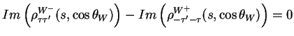
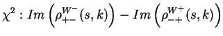
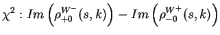
A further test of CP-invariance in the W-pair production process is given by the imaginary parts of the single W SDM elements. At tree level CP-invariance requires the following:
 |
(11.1) |
This equation gives a completely Model independent test of CP-violation
in the W-pair production process. Plots of the combinations of imaginary SDM
observables needed to test CP-invariance calculated from the 189 GeV data
can be seen in figure 11.1. No obvious deviations from zero
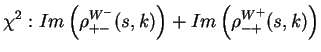
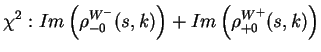
are observed. Calculating the ![]() for each plot, the following are obtained:
for each plot, the following are obtained:
 |
|||
 |
|||
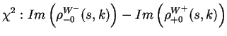 |
The ![]() includes both statistical and systematic uncertaintes. As each histogram contains eight degrees of freedom, these results are consistent with Standard Model expectations.
includes both statistical and systematic uncertaintes. As each histogram contains eight degrees of freedom, these results are consistent with Standard Model expectations.
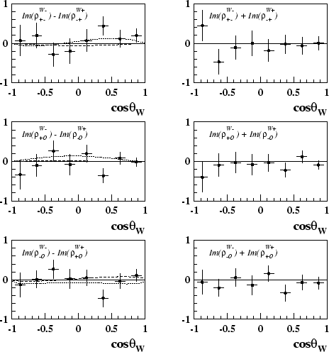 |
Also included in figure 11.1 are the plots that test for effects beyond tree level, as discussed in chapter 3, equation 3.48. Any deviations in
these plots could only be due to effects beyond tree level or CPT-violation. No
obvious deviations from zero are seen. Calculating the ![]() for each plot,
the following results are obtained:
for each plot,
the following results are obtained:
 |
|||
 |
|||
 |
These results do not give an indication of effects beyond tree level.