The Single W Spin Density Matrix

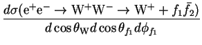
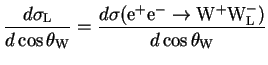
If only one of the W bosons in the W-pair is considered then the differential cross-section can then be written in terms of the single W Spin Density Matrix (SDM) [36,41]. For example, if only the ${\rm W}^{-}$boson is considered,

$$\frac{d\sigma({\rm e}^{+}{\rm e}^{-}\rightarrow{\rm W}^{+}{\rm W}... ... W}^{+}+f_{1}\bar{f}_{2})}{d\cos\theta_{\rm W}d\cos\theta_{f_{1}}d\phi_{f_{1}}}$$ (3.35)

$$=\frac{d\sigma({\rm e}^{+}{\rm e}^{-}\rightarrow{\rm W}^{+}{\rm W... ...cos\theta_{\rm W})D_{\tau_{1}{\tau^{\prime}}\!_{1}}(\theta_{f_{1}}\phi_{f_{1}})$$

Equation 3.35 is known as the 3-fold differential cross-section. The single W SDM completely describes the polarisation properties of one of the W bosons when the helicity of the other W boson has been effectively summed over. So the single W SDM is related to the two-particle joint density matrix as follows,

$$\rho^{W^{-}}_{\tau_{1}{\tau^{\prime}}\!_{1}}(s,\cos\theta_{\rm W}... ...{2}} \rho_{\tau_{1}{\tau^{\prime}}\!_{1}\tau_{2}\tau_{2}}(s,\cos\theta_{\rm W})$$ (3.36)

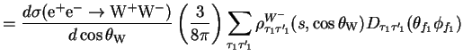
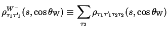
Like the two-particle joint SDM, the single W SDM has purely real diagonal elements and complex off-diagonal elements. The single W SDM contains nine elements, the diagonal elements of which are the probability of producing a W boson of helicity $\tau_{1}$, and so are normalised to unity,

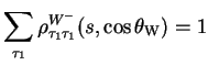
$$\sum_{\tau_{1}}\rho^{W^{-}}_{\tau_{1}\tau_{1}}(s,\cos\theta_{\rm W}) = 1$$ (3.37)

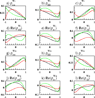
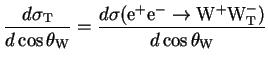
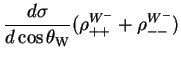
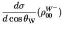
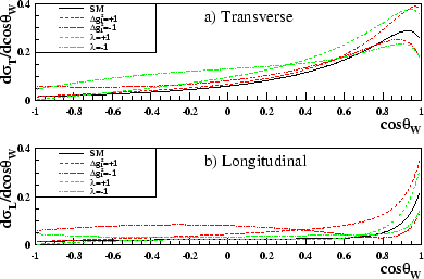
Examples of some of the real parts of the single W SDM elements can be seen in figure 3.11. The individual W polarised cross-sections, which are the differential cross-sections for producing a transversely (T) or longitudinally (L) W boson in the pair, where the other W boson can take any polarisation, can be written in terms of the single W SDMs. So for the polarisation of the ${\rm W}^{-}$ we have,

$$\frac{d\sigma_{\rm T}}{d\cos\theta_{\rm W}} = \frac{d\sigma({\rm e}^{+}{\rm e}^{-}\rightarrow {\rm W}^{+}{\rm W}^{-}_{\rm T})}{d\cos\theta_{\rm W}} = \frac{d\sigma}{d\cos\theta_{\rm W}}(\rho^{W^{-}}_{++}+\rho^{W^{-}}_{--})$$

$$\frac{d\sigma_{\rm L}}{d\cos\theta_{\rm W}} = \frac{d\sigma({\rm e}^{+}{\rm e}^{-}\rightarrow {\rm W}^{+}{\rm W}^{-}_{\rm L})}{d\cos\theta_{\rm W}} = \frac{d\sigma}{d\cos\theta_{\rm W}}(\rho^{W^{-}}_{00})$$ (3.38)

Figure 3.11: The real parts of the single W spin density matrix elements. The black line is the Standard Model case and the red (green) line is with an anomalous coupling of $\Delta g^{z}_{1}$$=+$1 ($-$1).

Examples of the individual W polarised cross-sections can be seen in figure 3.12. Shown, are the cross-sections for the Standard Model as well as those with various anomalous couplings implemented.

Figure 3.12: The analytical predictions of the individual W polarised differential cross-sections for the production of transverse and longitudinal W bosons. Examples of the Standard Model as well as some non-Standard Model cases are shown.