

![]()
![]()
![]()
![]()
![]()
![]()
![]()
![]()
8h HighSpeed TCP Transfer Across MB-NG - 22nd Feb 2003 ~ midnight
Purpose
The purpose of this test is to see the effects of a modified TCP stack across the MB-NG networking. The test was performed on a single stream for 8hours. This duration was chosen due to beaurocy.
Method
An implementation of HSTCP was installed on a stock 2.4.19 kernel. The implementation was by Gareth Fairey @ Manchester. It is available here. It was transfered using iperf set to socket buffers of 2m at both ends (optimal value is about 800k for this link) with logging (-i) of 1 second. It was recorded with web100 2.1a using a logging script called logvars which was set to record the web100 variables every second.
The transfer was between lon02 and man02 @ mb-ng.net.
The /proc/sys/net/route/flush was set to 1 to prevent ssthresh limitation.
Note that man02 is actually man03.
Results
sender log web100
recv log web100
Throughput
The average throughput throughout the 8h was reported as:
[ 3] 0.0-28800.0 sec 3362926026752 bits 934 Mbits/sec
Compared to the 918 achieved with StandardTCP (see here), it's not bad. The line rate achieveable with the link is limited to 1Gb/sec which roughly equates to about 947mbit/sec.
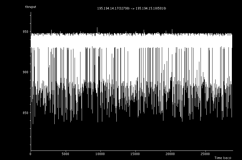
This graph shows the variation of throughput throughput the 8h.
And this graph shows the same but with web100. As you can see, the variation is not bad; at least it's a lot less variable than that with the vanilla tcp. This suggests that either we get less losses (causing reductions in the cwnd), or that if it's the same, the recovery is faster, hence more at the optimal value.
Looking at the cwnd values show that it grows to the same maxima value as the vanilla tcp does. However, whilst we got a wide band with vanilla tcp of 600,000 to 1.2e6, we get only 800,000 to 1.2e6 with hstcp. This implies that we get a larger window (on average) than with vanilla tcp - hence achieving slightly higher throughput.
This shows a zoomed view of the initial first 10 minutes of the transfer.
This shows the cwnd value for various throughputs for each sampled second in the test. There is almost none of the structure of the vanilla tcp here at all.
The above graphs show the cwnd values for various instbws for when there are no sendstalls. As you
| Wed, 23 July, 2003 13:07 |
This graphs shows the cumulative number of sendstalls as we progress through the transfer. We appear to get approximately 7-8 times the number of Sendstalls than with the vanilla tcp. This is most likely due to the fact that the AIMD algorithms are much more aggressive with HSTCP and hence creates tries to send more packets into the network. This in turn is trapped by the txqueuelen and signals to userspace (the tcp) to go into congestion avoidance.
[TODO: analyse effect of various txqueuelens on hstcp. Need to determine a way of measuring the packets]
At line rate, we can send at 1gb/sec. At 1538bytes (ethernet) - see table, we can achieve 1,000,000,000/(1538*8) pkts. This equals 81,274.38 pkts/sec maximum.
| Frame Part | Minimum Size Frame |
| Inter Frame Gap (9.6µs) | 12 Bytes |
| MAC Preamble (+ SFD) | 8 Bytes |
| MAC Destination Address | 6 Bytes |
| MAC Source Address | 6 Bytes |
| MAC Type (or Length) | 2 Bytes |
| Payload (Network PDU) | 1500 Bytes |
| Check Sequence (CRC) | 4 Bytes |
| Total Frame Physical Size | 1538 Bytes |
The distribution of pkts appears to be more sharp than with Vanilla TCP; maintaining a higher average number of pkts out.
This graph shows the occurances of when tcp is trying to push out more pkts than possible at line rate.
This graph shows the two regions in a different graph. We have the region in blue where the number of pkts out is greater than the line rate (calculated above), and red every else. The strange this here is that the blue area (greater than line rate) is actually only a compact region on the whole graph. Looking at the table, we have 5865 instances where the pktout is greater than the line rate (blue) and the rest 22936 below the line rate (red).
[TODO: Why are we getting sendstalls even though we supposedly do not send that many packets out?]
THis shows the cumulative number of congestion signals throughput the transfer. We get about 0.86 congestion signals per second. This is also far greater than the value obtained with the vanilla tcp here by about a factor of 5.
![]()
This shows the number of fast retransmit experienced on the link. The kink at ~11000secs can be attributed to a sudden cwnd of 0 that can been seen in the first graph. This basically means that so many packets were lost (or badly reordered) that the tcp window shrunk so much that the tcp had to retransmit them. TCP reponds by halving it's cwnd every time a packet is assumed lost and therefore given enough packets are assumed lost, then the cwnd dimishes and hence so does throughput.
Compared to the vanilla tcp run, the loss rates are almost the same (except for the kink) implying that the link's loss rate is still about 1e-5.
This graph shows the correlation between the loss of a packet (timeout) and another corresponding loss of the packet causing the cwnd to shrink. When a timeout happens, tcp actually instead of halving it's rate, will go back into slow start.
Hmm.. this graph shows the cumulative number of entries into slow start as shown by web100. This suggests that it almost constantly entering slow start at a rate of about 233 times per second! Given that the rtt is about 6ms, in one second, we get about 166 acks back if tcp were ping pong (which it isn't!).
Hmm...
At least the good news is that we enter congavoids more by about a facotr of 100. ie for every entry into slowstart, we see about 100 entries into congavoid.
Is this consistent with the loss rates?
This graph shows the correlation between the number slow starts at any instance and the number of send stalls for the same interval of one second. Each point represents that same time interval. There doesn't appear to be any correlation between the two variables - with slow starts occuring when there are not many sendstalls occuring. Should there be a relationship, the number of slow starts should increase with the number of sendstalls.
These two graphs show the rtt's from web100. Both graphs show the same thing but at different scales on the y axis. Just after 11,000 seconds, there appears to be a hugh increase in the rtt. This matches quite well to the second timeout value (from the timeout graph). The first timeout appears to be from the first increase in rtt as can be seen from the bottom rtt graph at 10,000 seconds.
This graph shows the affect of the rtt's against the min, max and cur RTO values.
This graph shows a magnified view of the above graph for the region of interest.
This graph shows that the profile of rtt's is quite sharp; peaking at about 8.7-8.8ms. (graph capped to 12ms).
This graph is interesting. Typically, for every 3 consequtive dupacks, we should enter fast retransmission. However, as it is highly possible that 3 dupacks do no arrive consequtively.
This shows the actual number of the packets and fastretrans per second rather than the cumulative. We can see that we get two bands:
- ~280 dupacks per second
- ~450 dupacks per second.
at an ave rtt of about 8.8 (see above graph), we get around 113 entire windows flowing through the system. (As one rtt represents roughly 1 window worth of data - and 1000/8.8 = 113).
| Wed, 23 July, 2003 13:07 |
Room D14, High Energy Particle Physics, Dept. of Physics & Astronomy, UCL, Gower St, London, WC1E 6BT