Proton Calorimetry/Experimental Runs/2017/Aug10-31
Experimental tests with Nuvia 10mm and 3mm scintillator sheets and Pravda CMOS stacked sensor.
Set-up of the MAPS sensor
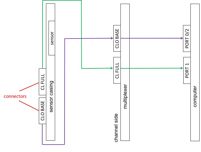
This section contains the instructions to take images with the MAPS sensor developed for the PRaVDA collaboration. In order to use the MAPS sensor, three components are essential:
- MAPS sensor integrated in board
- Multiplexer
- Computer with aSpect software
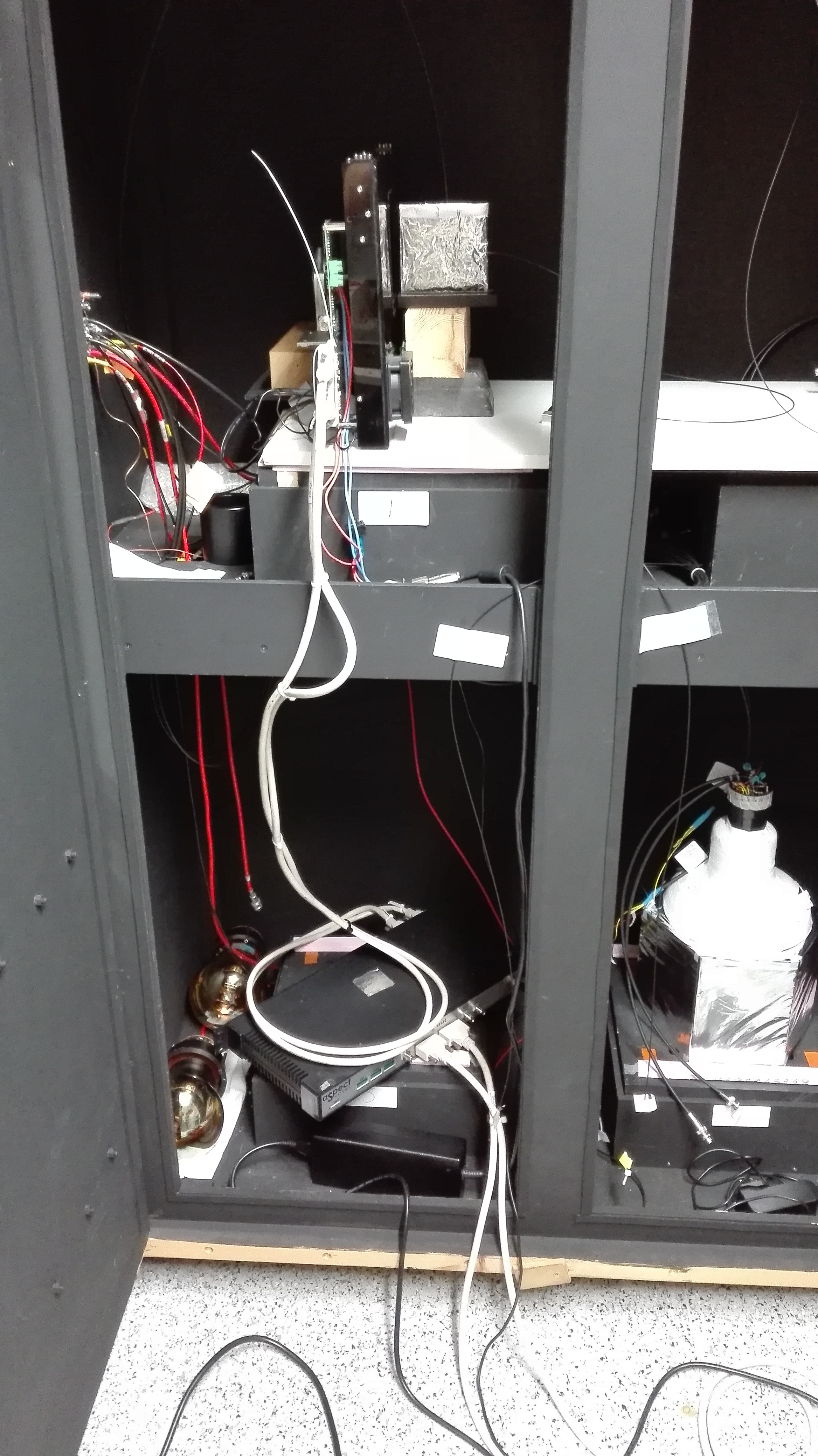
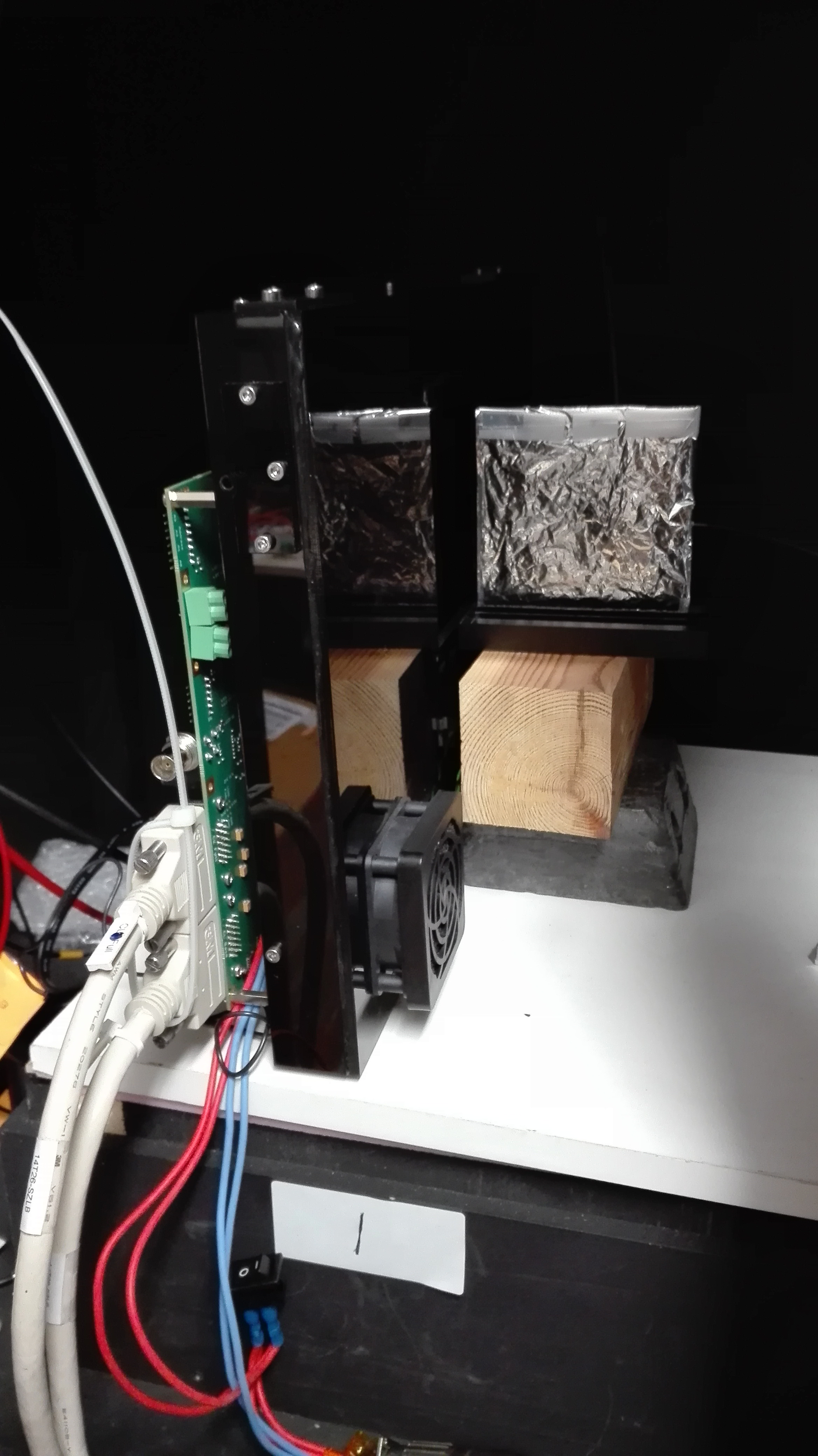
The MAPS sensor has to be set up in a light-tight box. Connect the board to the Multiplexer and the Multiplexer with the computer, using the labeled cables. "Full" has to be connected with port 1 on the computer. Remove the the aluminum foil in front of the sensor. It is important not to touch the MAPS sensor, especially while taking pictures when the bias voltage is switched on. Doing otherwise might destroy the sensor! Turn on the board and the multiplexer. Connect the LED with the scintillator sheet. Place the scintillator sheet in front of the sensor, the unwrapped side pointing towards it. Switch on the LED board. Set the settings of the LED, e.g. frequency=100kHz, pulse length=30ns, bias voltage=5V. Then switch on the LED.
.
.
.
Follow these steps to take an image with the MAPS sensor:
- Launch computer. Password: aSpect
- Some window will open automatically. In "Drive U Substitution" select first entry. Then press "substitute".
- Open "IDMate":
- In "DUT Grap" (find it in upper left corner) select "Init Testsystem" and press "play" button.
- TCP will show error message.
- Set settings:
- n21: Stream_master: value=1
- n32: CB111_En: value=1
- n46: BeamClk_En: value=0
- Confirm by pressing "Set all"
- Select "DUT init CT mode" and press play button.
- To record frames, select "Streaming Start" and press play. It will ask you to select a file name. After confirmation, frames are recorded.
- More important settings:
- n24: Set saving path for file.
- n26: Stream_repeats: set number of frames. "0" equals one frame, "1" equals two frames, etc.
- n28:Stream_daqtime: integration time of sensor in seconds. Must be an integer between 1 and 6.
- To exit IDMate, select "DUT Exit" and press play button.
- Files are stored in a binary format. In order to have a quick look at the output, use "Pravda file viewer".
- Select file in upper bar. Then press "Read file".
- Select "Image" button to see visualisation of the binary data.
- There is the possibility to export the data as .txt file or .tif image.
Analysis of binary data
There is a python script allowing to quickly plot and analyze the binary data generated by a MAPS sensor, written by Michaela Esposito. All necessary functions are collected in CMOS_functions.py. A minimum example of how to use those functions can be found in example.py.
The MAPS sensor will take 45 images per second. It is important to note that the first three images recorded by the MAPS sensor (numbered "-1", "0", and "1"), have to be discarded because of image errors. In addition, the upper five pixel rows of of each image show irregular behaviour and should be discarded in further analysis.
The 10 by 10 cm^2 MAPS sensor is decomposed into two independent sensors, each of a size of 5 by 10 cm^2. Both sensors are slightly shifted against each other, resulting in a shift in the images whenever both sensors are used.
10th August
On the 10th of August 2017, a first test of the MAPS sensor guided by Dr. Michaela Esposito took place at UCL. A scintillator sheet of 1cm thickness has been flashed by an LED. The distance between MAPS sensor and scintillator was about 1cm. The LED has been flashed at a bias voltage of 5V, a pulse length of 30ns and a frequency of 100kHz, corresponding to the maximum save settings to operate the LED.
A picture of the bright scintillator has successfully been taken using the MAPS sensor.
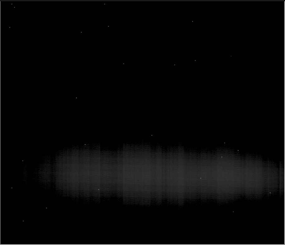
Single picture with background as it shown by the Pravda visualizer GUI.
After summing all 45 pictures taken in one second and subtracting the background measurement, the following image quality may be obtained:
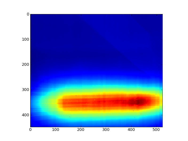
Summed background-subtracted picture 10mm produced with the python routine example.py.
A maximum of the light emission can be seen on one side of the scintillator sheet. This is due to an angle between the MAPS sensor and the scintillator sheet: The right edge is closer to the sensor then the left edge of the scintillator. In addition, another defect pixel row can be identified on the lower right hand side of the image.
14th August
On the 14th of August 2017, more tests of the MAPS sensor, using a 3mm thick scintillator sheet have been performed at UCL. The MAPS sensor successfully recorded a picture of the scintillator sheet flashed with an LED.
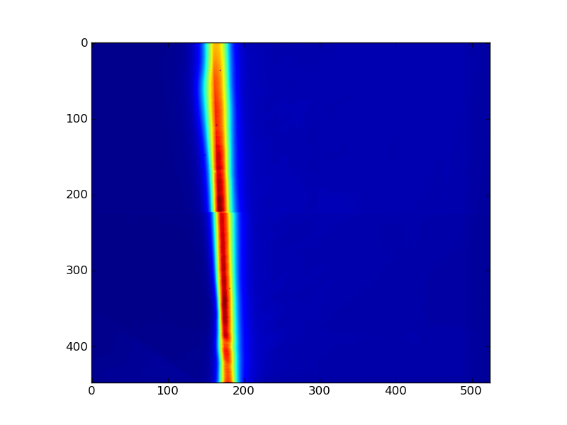
Summed background-subtracted picture 3mm produced with the python routine example.py.
The border between the two MAPS sensors can be identified easily. There is a small shift between both sensors, resulting in a shift in the centre of the image. In addition, a small gap between the two sensors can be seen. This is due to the five defect pixel rows at the upper edge of the lower MAPS sensor.