 Physics in a TeV linear Collider
Since the 1960s, most particle accelerators built accelerated particles along a closed, roughly circular path. This is a good design technique, as, firstly it allows to focus the particle and anti-particles using the same magnets; secondly the particles can be made to go round the accelerator several times to attain very high energies, and thirdly the beams can be made to cross several times, to obtain a maximal number of collisions.[1fgt accelerators]
But this design is limited by brehmsstrahlung radiation, the process by which a charged particle radiates a photon when its path is bent—which is nearly constant in a ring-shaped particle accelerator. The amount of emitted brehmsstrahlung is inversely proportional to the mass of the particles –so light particles such as electrons (e-), positrons (e+) and muons(μ) are much more affected. LEP(Large Electron-Positron collider), at 60GeV, attained a limit for electrons-positrons, after which the particles loose too much energy in each turn.
The only way to accelerate e+ and e- at significantly higher energy appears to be the construction of linear colliders, where particles are accelerated along a linear path.
Physics in a TeV linear ColliderThere are several compelling arguments[1worldwide LC study] for building a linear collider with energy range ~100GeV to 1TeV in the next few years. This is the timescale which will see the construction of the LHC (Large Hadron Collider ) at CERN in the LEP tunnel, which will attain energies of ~14TeV. The main aim for both a linear collider and the LHC is to find the mechanism which gives mass to gauge bosons and fermions, conjectured in the standard model to be the Higgs boson.
At the energies in question, the LHC will suffer from large backgrounds in Higgs production processes, as a consequence of being a hadron collider. This experimental difficulty will make the measurements of Higgs quark couplings, and Higgs self-couplings difficult. Electrons and positrons, as point-like particles, give a much cleaner signal, enabling the direct measurement of Higgs quantum numbers, and of its finer characteristics and threshold (the only parameter not predicted by the standard model is its mass, hints of which have been detected at LEP between 144 and ~200 GeV.) It is expected that a Higgs boson could be produced with only 2-3 other products in a linear e+e- collider, as opposed to numbers of the order of 100 in LHC.
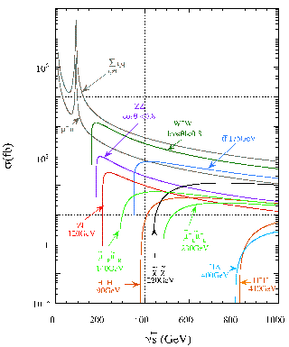
Fig a: Interesting cross sections
at a 1TeV linear Collider [jlc homepage]
Beyond the standard model, super symmetry (SUSY) theories predict the existence of supersymmetric sparticles, mirroring particles in supersymmetric space and time dimensions. Effects are predicted in the 100-1000GeV range, either directly from sparticles of in this mass range, or indirectly from heavier sparticles; linear collider measurements could give information to select good SUSY theories.
As part of its programme, and particularly relevant for this project, a linear collider would be used for top quark physics (precise measurement of all top quark parameters), and W and Z boson precision measurements.
 TESLA
TESLA
This project is mainly intended as a study for TESLA the next generation linear accelerator planned in DESY, Hamburg. TESLA (Tera-electron volt Energy Superconducting Linear Accelerator), is one of the contenders for a next generation linear collider. The main others are NLC (Next Linear Collider, Stanford[nlc homepage]), JLC (Japan[jlc homepage]) and in the longer term, CLIC at CERN[clic homepage](at a higher 3-5 TeV energy range.)
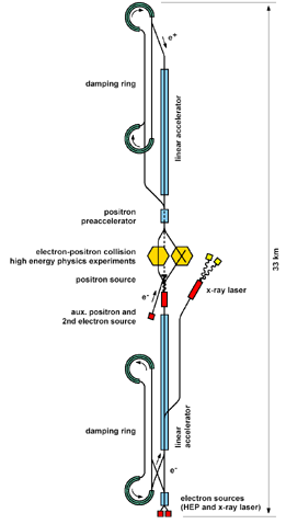
TESLA is planned to accelerate electrons and positrons to a center of mass energy of 500GeV at first. In a second phase, energies of 800GeV-1TeV will be attained. The setup is over 30km in length, and the acceleration is carried out using superconducting niobium RF cavities, cooled at 2K by liquid helium. These allow very high acceleration gradients ( more than 30MV/m), and allow the acceleration and conservation of very small bunches.
A major challenge of TESLA is to produce high-luminosity beams: this means achieving very small spot sizes by concentrating the particles into bunches of length of a few hundred μm, and of widths one thousand times less. The bunch populations would average 1010 particles, and the bunches have to be damped to reduce emittance in large damping rings, as in fig. b. opposite.
In addition to e+e- collisions, TESLA has the capability of colliding e-e-(which can be used to search for heavy Majorana neutrinos), as well as γe- and γγ photon collisions, which would test fundamental QCD predictions of the F2γ photon structure function.
Fig b:TESLA overall layout sketch,
[1tesla tdr], II-7.
In practice, when the beam is run at given energy, some particles lose energy before the collision for several reasons. The range of collision energies is distributed in a spectrum, sharply peaked, with more than 65% of events with 0.1% of nominal energy: this distribution is referred to as the e+e- luminosity spectrum, ∂L/∂√S.
It is hoped that by using physics processes known as bhabha scattering, the energy spectrum can be reconstructed with an accuracy of 0.1%. This would be sufficient for top quark physics, whereas investigation of W mass would require an accuracy better by an order of magnitude: 0.01% in the luminosity spectrum.[cinabro jeju talk],[1miller boogert 02]
The three main processes that contribute to an energy loss are machine beamspread, beamstrahlung, and Initial State Radiation. They are detailed below:
This is the smallest source of energy loss. It is induced by the intrinsic energy spread of the e- and e+ produced by the machine, and it is an inescapable process.
Because of the process by which the electrons are used to produce the positrons, the latter will have a lower machine energy spread. The value for the positrons is 0.05%, and for the electrons it is 0.15%. This effect is unlikely to be gaussian.
We can already see the difficulty in reconstructing a spectrum to 0.1% accuracy, when the electrons have an intrinsic 0.15% energy spread.
number of events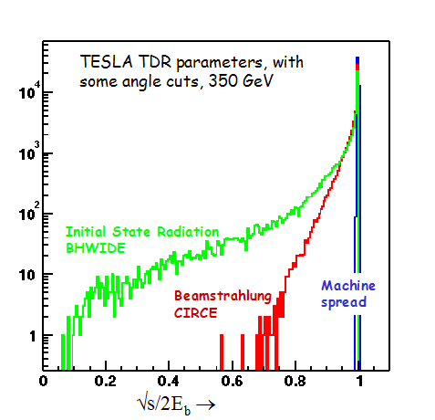
beamstrahlung is the name of the energy loss that electrons and positrons experience when the particles of one beam interact with the electromagnetic field of the opposite bunch. It is equivalent to brehmsstrahlung, which is caused by bending the trajectory of a charged particle, and has the same spectrum; in effect they are both caused by accelerating the particle.[1schulte thesis]
This is quite a large effect in an accelerator like TESLA[cinabro], as charges in the bunches are very concentrated due to small beam sizes.
Initial State Radiation (ISR) is a consequence of QED. At any given time, one of the beam particles can radiate a photon, thus losing energy.
It can be calculated to great accuracy, and would not need to be measured if it were the only effect present. To calculate it, some QCD cross sections have to be taken into account; we used BHWIDE, a wide angle bhabha scattering simulation program (fist developed in LEP[1bhwide page].)
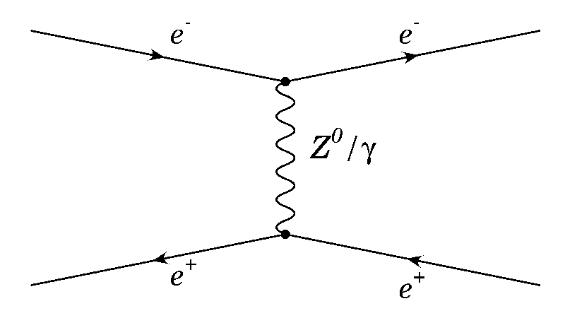
Fig e: t-channel bhabha scattering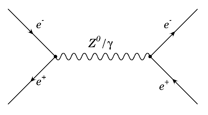
 Fig
d: s-channel bhabha scattering
Fig
d: s-channel bhabha scattering
The reasons why this is the preferred process to estimate √s are that it has better statistics than the physics channels (400 times the μμ rate in our angular range), and it has a good energy resolution. At small angles, the error on on √s grows, becoming more significant below 0.1 radians.
The process is basically described by the exchange of a virtual photon, or a Z0 boson. In our angular range, the s-channel dominates, and the Z0 contribution is small.[lep precision physics]
From outgoing particle angles the momentum loss can be estimated, and thus the energy loss from nominal energy, under the assumptions that a.) only one photon has been radiated and b.) it was radiated along the beam.
The distribution of √s will then give the luminosity spectrum, ∂L/∂√s.
e+ γ,
emitted
along the beam
θ2
e- θ1
z
axis (beampipe) Fig f: bhabha scattering event
schematic diagram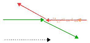


The angles θ1 and θ2 are defined as shown in fig. f. The acollinearity angle θA is equal to the difference of θ1 and θ2 ( θA = θ1 - θ2 ).
The angle θ is taken as the average between θ1 and θ2. For small acollinearity ( θA<< θ), we have θA=(Δp/pb)sinθ, where Δp = p1-p2, the momentum difference between the two particles at collision.
The quantity needed is √S ≈2pnom - θApnom/sinθ by this estimate.
Considering the error: for small θA , if the error is Gaussian, σ√s≈ σΔp ≈ σθApb/sinθ ≈ √ σpb.
So the error increases as the scattering angle θ approaches 0, which implies better luminosity resolution for slightly liarger angles.
This approximation can be derived directly from bhabha scattering kinematics (cf. Appendix B): if the 4-momenta of an electron and a positron are added to find the center of mass energy, and it is assumed that a.) one photon is radiated in the direction of the beampipe, and b.) the paths are coplanar, then some algrebra will yield:
√s ≈ √cot (θ1/2) cot (θ2 /2) cf. Appendix B for algebra.