The initial method to extract the lag was to approximate the heating/cooling as sin functions and use the properties of phase offsets to get the lag. If the RS and DCS temperature are paramterized as y1=A1*sin(x+phi1) and y2=A2*sin(x+phi2) then by plotting the asin(y1) vs asin(y2) it is possible to get rid of the x term and have just the phase (offsets) plotted against each other. The problem with this is two-fold:
1) The amplitudes of A1 and A2 change and they don't scale well i.e. A1 = 1.7*A2. This was shown by earlier work in the Temperature 3 presentation. There is some linear correlation in the DCS vs RS Temp slopes but the error on the histograms that would define this amplitude coefficient is too large to be reasonable. This means that between days there is enough fluctuation in the heating/cooling (amplitude) slopes that would essential ruin this analysis. The scaling rate needs to be known in order to make sure that y1 and y2 can be scaled to a value less than 1.
2) The more dominant issue is that the plots aren't nicely sinusoidal. In fact they aren't nicely anything. In a completely enclosed space devoid of random temperature changes from doors opening/closing or drafts, modeling becomes possible. In the meantime the data is routinely jumpy and this makes any sort of mathematical approximation approach to this problem extremely difficult.
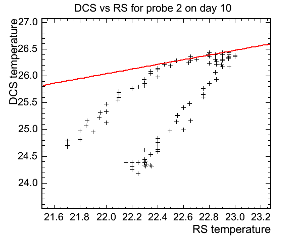
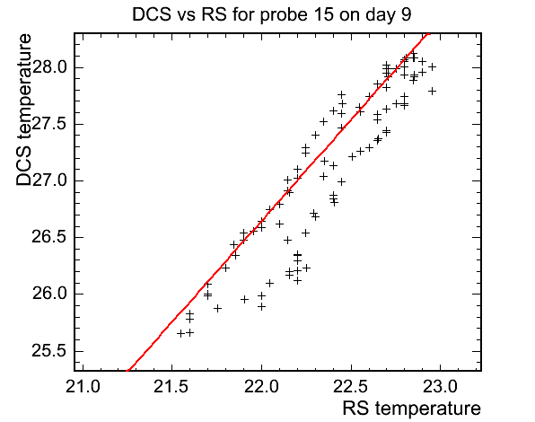
The method that I have thought to employ that avoids this pitfalls is that of a running average along X points. There are plots of DCS vs RS that do show a rounded peak and a slight separation between heating and cooling in so far as they do not perfectly make a straight line. If there were to be no lag between the DCS and RS temperature then DCS vs RS would produce a straight line. This is because as soon as one started to cool, so would the other.
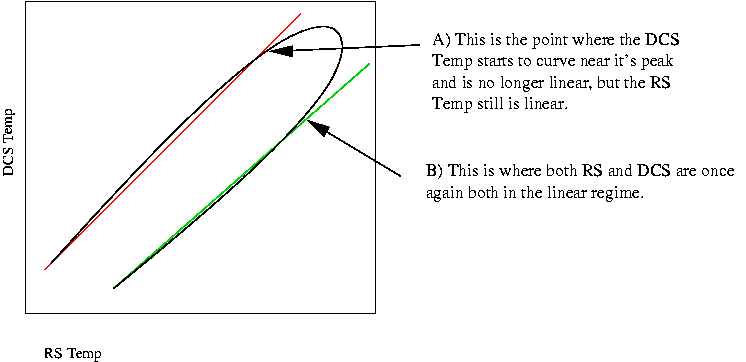
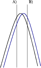
To the left of line/point A both the
DCS
(Black) and RS(Blue) are linear and so plots of DCS vs RS will also be
linear. The DCS starts to become non-linear first and its gradient at
this point starts to decrease, while the RS Temp continues being
linear. This causes the curved section of the semi-elliptical DCS vs RS
plot to being. When
the DCS becomes linear again, at some point near the maximum of the RS
Temp, it is the RS Temp that is now non-linear, and thus the DCS vs. RS
is still in the curved section at the tip of the semi-ellipse. The DCS
vs RS plot becomes linear once again when both RS and DCS are in their
linear regime, the region to the right of point B, so the offset
is 1/2 the time between points A and B.
The running average idea is to take X
points and have them move along this path between points A and B. From
work in the Temperature 3 presentation I have found the avg. slopes of
all the probes for both heating and cooling. So I am looking for the
point at which the running avg. slope leaves the heating slope and
calling that point A. Then letting the X points increment along find
out how long it takes for the running avg. slope to be equal to the
cooling slope and calling that point B. God willing (B-A)/2 will
give the offset.
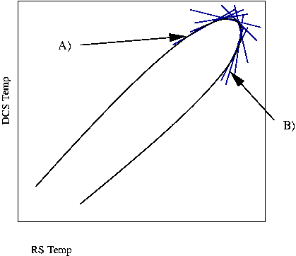
This is an improvement on using mathematical modelling because it does not rely on the data to be in a near perfect shape. As long as there is an some curvature at the the top of the DCS vs RS plot that will suffice for this method.
This is an improvement on using mathematical modelling because it does not rely on the data to be in a near perfect shape. As long as there is an some curvature at the the top of the DCS vs RS plot that will suffice for this method.
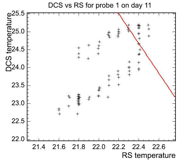
Initial results
The code is mostly in place now, and the some initial plots show that the points A and B can be found, but refining the parameters that go into the method is now needed. The current incarnation finds the points A and B and then calculates a line between the two. Another loop is run over all the data and finds all the points that lie 'above' this line and counts them multiplies by 5 to get the minutes. I've been examining the data over 4 good days that I've found that do not have anomolous dips and the data is quite varied. Even examining single probes gives results that by quick eye-inspection do not seem correct. i.e. For probe 0 the over days 8-11 the RMS is ~12 minutes and the lag is 128 minutes, using the histogram data. Without futher ado, here are the plots.
The good:
The not so good:
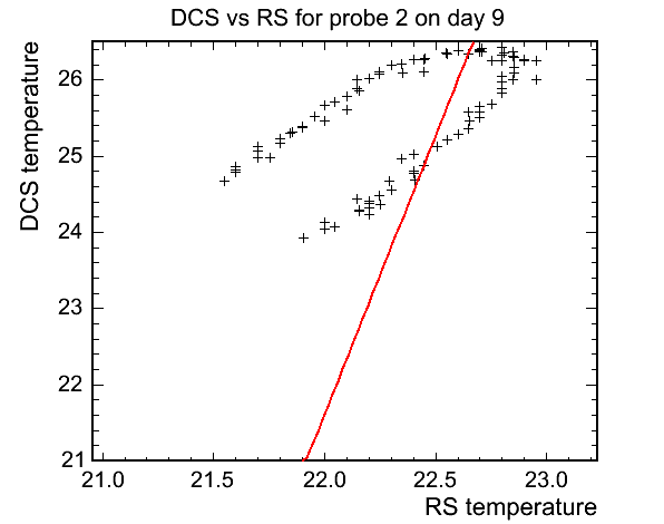
And the Bad: