Stability of the $\chi ^{2}$ fit

In this appendix the stability of the $\chi ^{2}$ fit method is discussed and tested. When a $\chi ^{2}$ is formed containing a number of highly correlated observables it can become unstable. As the correlation tends to unity the $\chi ^{2}$ can fail and thus not give a meaningful result.

In chapter 6 the $\chi ^{2}$ fit used in the TGC calculations was tested extensively and found to be reliable. A further test can be performed where one of the diagonal SDM elements is omitted from the fit, this will then remove the problem of highly correlated elements. As the diagonal elements are highly correlated, this omission of one of them from the fit should produce little change in the fit results. In this appendix all fits are performed without the inclusion of $\rho_{++}$. This was an arbitary choice of SDM element to remove. It was found that the same result was yielded independent of which diagonal element was omitted from the fit.

All tests in this appendix were performed using only the BILGOU reweighting scheme, although similar tests were performed with the WVCXME reweighting scheme and the results were found to be compatible to those given here.

Figures B.1 and B.2 show the bias fits performed to Monte Carlo samples with various anomalous couplings and figures B.3 and B.4 show the fits to many Monte Carlo subsamples along with the pull distributions. All these results are consistent with those given in chapter 6

Figure B.1: Bias plots of the CP-conserving TGC fits using the BILGOU reweighting scheme. The first column is the fit to the SDM elements excluding $\rho_{++}$, the second column is the fit to the W production angle, and the third column is the combined fit. The solid line represents the perfect fit. The red points represent the expected statistical error on the data.

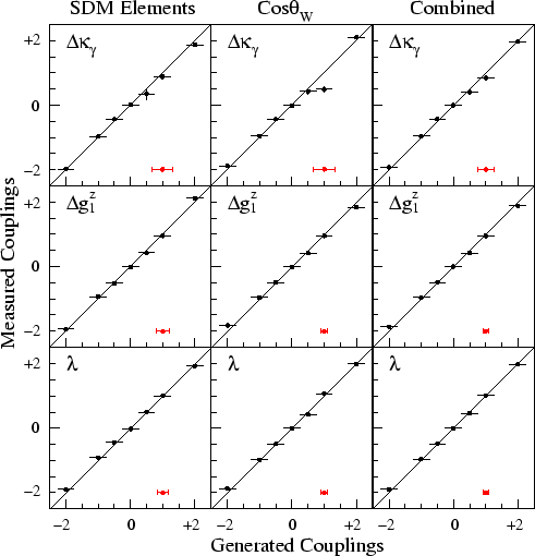Figure B.2: Bias plots of the CP-violating TGC fits using the BILGOU reweighting scheme. The first column is the fit to the SDM elements excluding $\rho_{++}$, the second column is the fit to the W production angle, and the third column is the combined fit. The solid line represents the perfect fit. The red points represent the expected statistical error on the data.

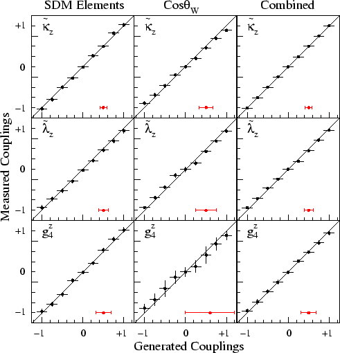Figure B.3: Combined fit results to 139 subsamples of Standard Model EXCALIBUR Monte Carlo. The BILGOU reweighting scheme was used in the fits. The widths of the distributions of the plots on the left side represent the expected error for the analysis for the corresponding coupling parameters. The width of the pull distributions, the plots on the right side, should be compatible with unity if the statistical error is reliable. All fits excluded $\rho_{++}$

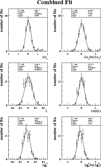Figure B.4: Combined fit results for the CP-violating couplings to 139 subsamples of Standard Model EXCALIBUR Monte Carlo. The plots on the left are the distributions of fitted values and the plots on the right are the pull distributions. All fits excluded $\rho_{++}$.

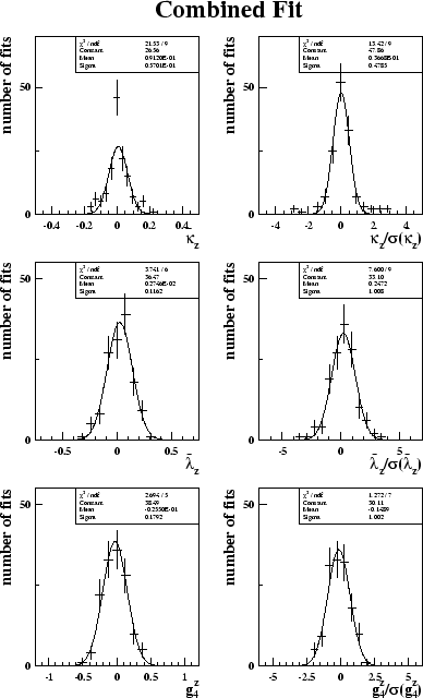The expected statistical errors calculated using the fit method excluding $\rho_{++}$, are shown in table B.1. They are equivalent to the values calculated in chapter 6.

Finally the actual values of the TGCs calculated from the data are shown table B.1. These are consistent with those calculated in chapter 7. Once systematic uncertainties are included a number of the results differ very slightly from those quoted in chapter 7, this is expected due to the less than exact way the systematic uncertainties are included in the $\chi ^{2}$ fit. The differences are still much less than the statistical precision of the results. 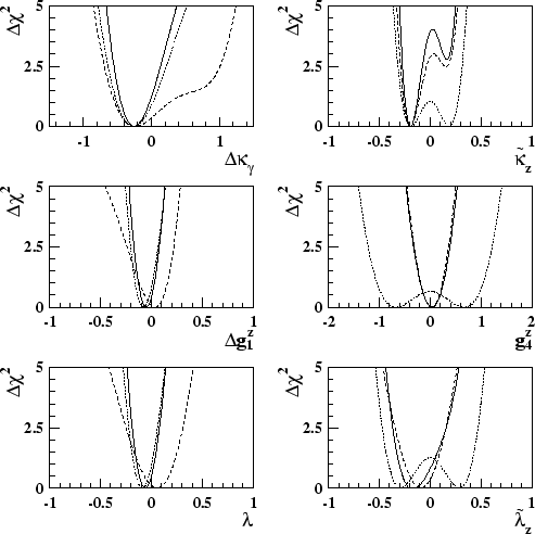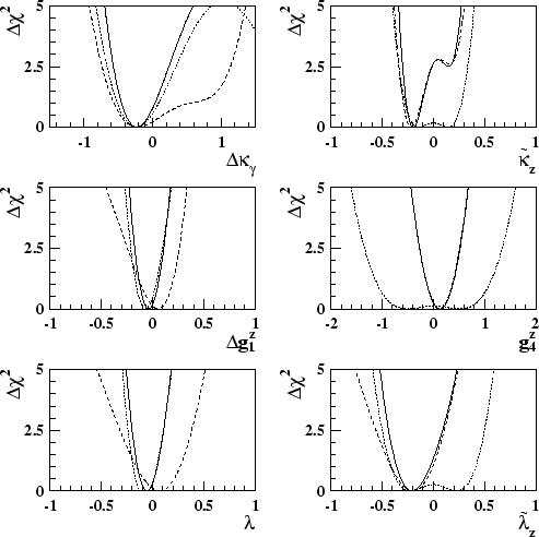The $\chi ^{2}$ plots for these fits can be seen in figures B.5 and B.6.

This appendix thus verifies the correctness of the $\chi ^{2}$ fit method used in the thesis and indicates that the high correlations between the SDM elements does not introduce instabilities in the $\chi ^{2}$ at the precision achievable with the LEP2 data.

Figure B.5: The $\chi^2$ plots for the fits to the CP-conserving and CP-violating anomalous couplings. For the CP-conserving couplings the dashed line is the fit to just five real SDM elements, for the CP-violating couplings it is the fit to eight SDM elements. The $\rho_{++}$ observable has been omitted. The dotted line is the fit to just the $\cos\theta_{\rm W}$ distribution. The solid line is the combined fit.

Figure B.6: The $\chi^2$ plots for the fits to the CP-conserving and CP-violating anomalous couplings. For the CP-conserving couplings the dashed line is the fit to just five real SDM elements, for the CP-violating couplings it is the fit to eight SDM elements. The $\rho_{++}$ observable has been omitted. The dotted line is the fit to just the $\cos\theta_{\rm W}$ distribution. The solid line is the combined fit. All fits include systematic uncertainties.