W Boson Decays

As W bosons are massive vector bosons they only have a very short lifetime. This means that within the OPAL detector the W-bosons are never directly observed, only their decay products are measured. W bosons decay into two fermions. A ${\rm W}^{-}$can decay into a lepton and anti-neutrino or a quark anti-quark pair. The branching ratios for each of these decays have been measured at OPAL from the W-pair production process [66], and is found to agree well with theoretical predictions [12] for the Standard Model and the world average [5]. The branching ratios calculated from all data collected at OPAL, assuming lepton universality to calculate the q $\bar{\rm q}$ branching ratio, is given below. In each case the first error is statistical and the second systematic.

$${\rm Br}({\rm W} \rightarrow {\rm e}\bar{\nu}_{\rm e}) = 0.1046 \pm 0.0042 \pm 0.0014,$$

$${\rm Br}({\rm W} \rightarrow \mu\bar{\nu}_{\mu}) = 0.1050 \pm 0.0041 \pm 0.0012,$$

$${\rm Br}({\rm W} \rightarrow \tau\bar{\nu}_{\tau}) = 0.1075 \pm 0.0052 \pm 0.0021,$$

$${\rm Br}({\rm W} \rightarrow {\rm q}\bar{\rm q}) = 0.6832 \pm 0.0061 \pm 0.0028.$$

With each W boson being able to decay into a lepton and neutrino or two quarks, this means that there are effectively three possible final states; Two leptons and two neutrinos, $\ell\bar{\nu}_{\ell}\bar{\ell}\nu_{\ell}$, known as the leptonic channel. Two quarks and two anti-quarks, q $\bar{\rm q}$q $\bar{\rm q}$, known as the hadronic channel. Finally there is a final state of a lepton, a neutrino, a quark and an anti-quark, $\ell\bar{\nu}_{\ell}$q $\bar{\rm q}$, known as the semi-leptonic channel. The branching ratios for these three channels given in [12] are, 45.6%, 10.5% and 43.9% respectively.

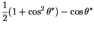
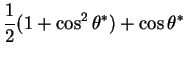
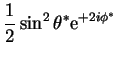
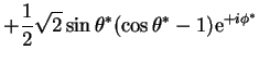
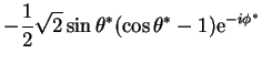
As the decay of W bosons into fermions has been well studied and understood and is believed to proceed via the standard V$-$A coupling, it is possible to predict the angular distribution of the decay fermions if the helicity of the W boson is known. The dependence of the angular distribution of the fermions, in the W boson rest frame, on the helicity of the W boson are given by the so called D-functions [36]. The explicit form of these D-functions is given in equation 3.26, where $D_{\tau^{\prime}\tau}(\theta^{*},\phi^{*}) = D_{\tau\tau^{\prime}}^{*}(\theta^{*},\phi^{*})$.

$$D_{++} = \frac{1}{2}(1+\cos^{2}\theta^{*}) - \cos\theta^{*}$$

$$D_{--} = \frac{1}{2}(1+\cos^{2}\theta^{*}) + \cos\theta^{*}$$

$$D_{00} = \sin^{2}\theta^{*}$$ (3.26)

$$D_{+-} = \frac{1}{2}\sin^{2}\theta^{*}{\rm e}^{+2i\phi^{*}}$$

$$D_{+0} = +\frac{1}{2}\sqrt{2}\sin\theta^{*}(\cos\theta^{*} - 1){\rm e}^{+i\phi^{*}}$$

$$D_{-0} = -\frac{1}{2}\sqrt{2}\sin\theta^{*}(\cos\theta^{*} - 1){\rm e}^{-i\phi^{*}}$$

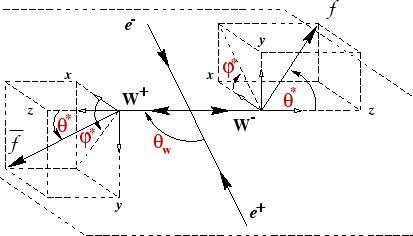
In the above equations $\theta^{*}$ is the polar angle of the decay fermion in the W rest frame and $\phi^{*}$ is the azimuthal angle of the decay fermion in the W rest frame, as illustrated in figure 3.9.

Figure 3.9: Production and decay angles of W bosons.

Knowing how the decay fermions couple to the W bosons of different helicity and also how the W bosons are produced in the W-pair through the helicity amplitudes, (3.18), an analytical expression for the differential cross-section of the process ${\rm e}^{+}{\rm e}^{-} \rightarrow {\rm W}^{+}{\rm W}^{-} \rightarrow f_{1}\bar{f}_{2}f_{3}\bar{f}_{4}$ may be written, (3.27). Where $\theta_{f_{1}}$ and $\phi_{f_{1}}$ are the ${\rm W}^{-}$ decay angles analogous to $\theta^{*}$ and $\phi^{*}$ respectively. $\theta_{\bar{f}_{4}}$ and $\phi_{\bar{f}_{4}}$ are the ${\rm W}^{+}$ decay angles analogous to $\theta^{*}$ and $\phi^{*}$ respectively. Br(X $\rightarrow$ a $\bar{\rm b}$) denotes the branching ratio for that process.

$$\frac{d\sigma({\rm e}^{+}{\rm e}^{-} \rightarrow {\rm W}^{+}{\rm ... ...d\cos\theta_{f_{1}}d\phi_{f_{1}}d\cos\theta_{\bar{f}_{4}}d\phi_{\bar{f}_{4}}} =$$

$${\rm Br}({\rm W}^{-}\rightarrow f_{1}\bar{f}_{2}){\rm Br}({\rm W}... ...f}_{4})\frac{\vert\vec{P}\vert}{16\pi s\sqrt{s}}\left(\frac{3}{8\pi}\right)^{2}$$

$$\times \sum_{\lambda\tau_{1}{\tau^{\prime}}\!_{1}\tau_{2}{\tau^{\prime}}... ...}_{{\tau^{\prime}}\!_{1}{\tau^{\prime}}\!_{2}}(s,\cos\theta_{\rm W})\right]^{*}$$ (3.27)

$$\times D_{\tau_{1}{\tau^{\prime}}\!_{1}}(\theta_{f_{1}},\phi_{f_{1}})D_{\tau_{2}{\tau^{\prime}}\!_{2}}(\pi-\theta_{\bar{f}_{4}},\phi_{\bar{f}_{4}}+\pi)$$

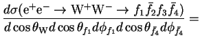
This equation is the differential cross-section in terms of the ${\rm W}^{-}$ production angle, $\cos\theta_{\rm W}$, the production angles of the particle from the ${\rm W}^{-}$ decay in the ${\rm W}^{-}$ rest frame, $\theta_{f_{1}}$, $\phi_{f_{1}}$, and the production angles of the anti-particle from the ${\rm W}^{+}$ decay in the ${\rm W}^{+}$ rest frame, $\theta_{\bar{f}_{4}}$, $\phi_{\bar{f}_{4}}$. Thus it is known as the 5-fold differential cross-section.

With a final state of four fermions all the possible final helicity states interfere with one another, so it is no longer meaningful to speak of TT, LL or TL final helicity states. The subscripts on the D-functions, shown in equation 3.26, do not indicate the spins of the two separate W bosons, but rather are both for a single W boson. In the 5-fold differential cross-section the helicity amplitude is multiplied by the complex conjugate of another helicity amplitude which has different subscripts. The $\tau_{1}$ and $\tau_{1}^{\prime}$ both refer to the ${\rm W}^{-}$ and so it can be seen that the first D-function relates to the ${\rm W}^{-}$, and intuitively the second D-function must relate to the ${\rm W}^{+}$. As the sum runs over all four $\tau$s this immediately implies there must now be 81 terms for each $\lambda$ helicity in the sum, rather than the nine seen in equation 3.25.

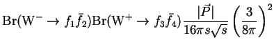
Upon integration of the D-functions over the W decay angles the following is obtained:

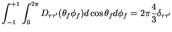$$\int^{+1}_{-1}\int^{2\pi}_{0} D_{\tau\tau^{\prime}}(\theta_{f}\phi_{f})d\cos\theta_{f}d\phi_{f} = 2\pi\frac{4}{3}\delta_{\tau\tau^{\prime}}$$ (3.28)

Integrating the 5-fold differential cross-section over both the ${\rm W}^{-}$ and ${\rm W}^{+}$ decay angles will thus retrieve the W-pair production cross-section as given in equation 3.25.