As mentioned in the previous chapter, higher energy accelerators are required to investigate the TeV energy scale. To complement the new generation of hadronic colliders, a leptonic collider is required, and to accelerate leptons to the required energy, a linear collider is needed. Currently, the highest energy linear accelerator is the SLAC Linear Collider (SLC), which ran from 1989 to 1998 and used 46 GeV electron and positron beams [17]. While the next generation of colliders will use the same principles of operation as the SLC, a large number of improvements are required to reach the required beam energies.
There are a number of different proposed designs for a next generation linear collider, all with the goals of achieving higher energies and luminosities than any of the previous machines. Each design is broadly associated with a particular accelerator laboratory and have the following titles (see the various references for more information):
The TESLA design is unique in that it makes use of superconducting niobium accelerating cavities, whereas each of the other designs uses ‘warm’ (i.e. room temperature) copper cavities; as a result, it also uses a substantially different bunch structure and damping ring design [22]. CLIC is intended as a ‘next-next generation’ accelerator, to take advantage of a number of developments necessary for the other accelerators; it is also the only accelerator to make use of the ‘two-beam’ accelerator concept and is intended to run at the much higher Centre-of-Mass (CMS) energy of 3 TeV [21]. The NLC and JLC, however, are very similar in design, and follow on conceptually from advances made in the design and construction of the SLC. There is also a considerable amount of ‘cross-pollination’ of personnel and technologies between the two collaborations. The remainder of this chapter will describe the generic design of the linear collider, with a focus on the design of the NLC. Some of the design parameters for the initial design of the NLC, and the proposed upgrade (Stages 1 & 2), are shown in Table 2.1 (each of these parameters is explained in the remainder of this chapter).
|
|||||||||||||||||||||||||||||||||||||||||||||||||||||||||
|
An accelerator is made up of a number of discrete sections, each of which accomplishes a different task. A brief overview of these sections is now given: more detail on beam dynamics and acceleration and the interaction region is provided in Sections 2.2-2.4.
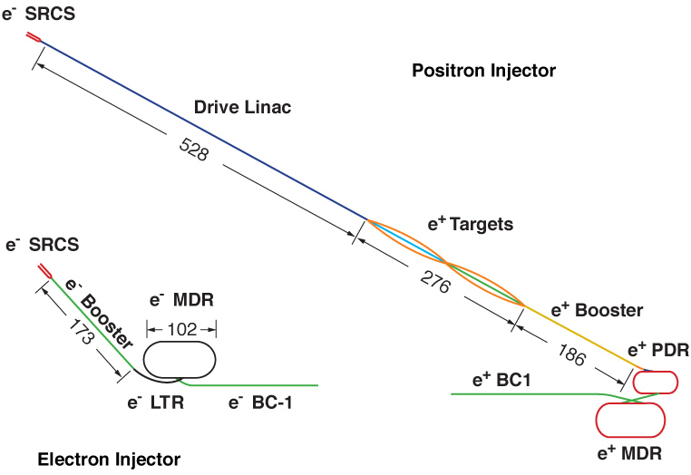
Although the bulk of the accelerator is made up of RF cavities to accelerate the charged particles up to the required energies, the front end of the accelerator is dedicated primarily to the production and collection of electrons (or positrons): this section is referred to as the Injector. The basic role of the injector is to produce the high quality particle beam that is to be used for acceleration within the main linac. The electron and positron injectors for the deep-bored-tunnel design of the NLC10 are shown in Fig. 2.1; the figure also shows the general layout of the damping rings: these are dealt with separately in Section 2.1.2. The other components that make up the injector are the source, a pre-accelerator, bunch compressors and various collimation systems [13].
| Figure 2.1: The electron and positron injector complexes for the deep-bored-tunnel design of the NLC [13]. The abbreviations used are as follows: SRCS – electron sources; BC-1 – 1st stage bunch compressor; LTR – Linac-to-Ring; PDR – Pre-Damping Ring; MDR – Main Damping Ring; dimensions are given in metres. |
The source, as its name would suggest, is the first stage in creating a usable particle beam. There are two main ways to create the large quantity of electrons that are required for both the electron and positron source, based on thermionic and photoelectric emission [23]. A high voltage DC thermionic gun uses a heated cathode to produce electrons, which are then initially accelerated with a DC voltage. A series of solenoids is then used to constrain these electrons and compensate for the natural tendency of the trajectories of similarly charged particles to diverge (an effect referred to as ‘space charge’), which would result in a rapid increase in beam spot size [24].
The electron source for the NLC actually makes use of the second method of electron emission: the photoelectric effect. A laser is directed onto a Gallium-Arsenide semiconductor photocathode: the photoelectrons produced are then accelerated in the same fashion as before. This method of electron production allows the selection of the polarisation of the resultant electron beam. Since one is able to choose the polarisation of the photons in the laser beam, the resultant emitted photoelectrons are also polarised, resulting in an electron beam with better than 80% polarisation [6]. A pre-accelerator is then used to further accelerate the beam, with successively higher frequency accelerating cavities (for more details, see Section 2.3). This causes the beam to bunch at the desired bunch spacing — in the case of the NLC, a pair of 714 MHz bunchers is used, setting the bunch spacing at 1.4 ns: the full bunch train consists of 192 bunches of 8×10⁹ electrons, with a full train length of 266 ns. An S-band accelerator, at 2856 MHz, is then used to further accelerate the beam to 2 GeV for injection into the main damping ring (see Fig. 2.1).
A second electron gun is used to produce the electrons that are required to create the positrons for the opposing beam. 6 GeV electrons are accelerated onto a Tungsten-Rhenium (WRe) target, causing electromagnetic showers within the target: the positrons produced by these showers are then collected and accelerated by an L-band linac (1428 MHz) to 1.98 GeV for injection into the positron pre-damping ring [13].
While it is undoubtedly important to produce bunches with a large number of particles, it is perhaps the size of these bunches that is the dominating factor in producing a high luminosity. For a linear collider, the luminosity, L, is defined as:
| (2.1) |
for beam energy E, number of particles per bunch N, number of bunches per train n, machine repetition rate f and beam power P [18]. HD is the beam pinch enhancement, resulting from the interaction of two oppositely charged bunches (see Section 2.4.3); σx* and σy* are the horizontal and vertical (r.m.s.) beam dimensions at the IP11. As such, since the luminosity is inversely proportional to the CMS energy (2E), it is imperative that the luminosity loss caused by going to higher energies is countered by a corresponding decrease in the spot size at the IP.
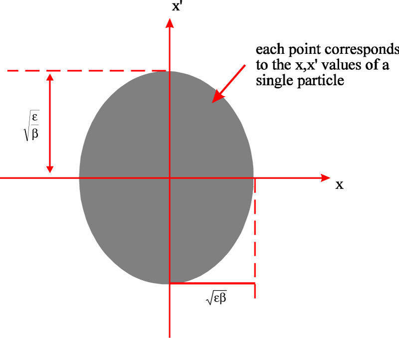
| Figure 2.2: A transverse phase space plot for a large number of particles in a particle beam [25]. The area of this phase space plot is defined as the (horizontal) emittance of the beam, εx; β is the beta function and is defined in Section 2.2.2. |
In order to produce a minimum spot size, it is necessary to minimise the horizontal and vertical emittance of the beam. The emittance is a measure of both the physical transverse size of the beam, x, and its divergence i.e. the angle12 of each particle trajectory within the beam, x′. If one plots the position versus angle of every particle within the beam, as shown in Fig. 2.2, this forms an ellipse in transverse phase space. The area of this ellipse is defined as the emittance of the beam: it is denoted by
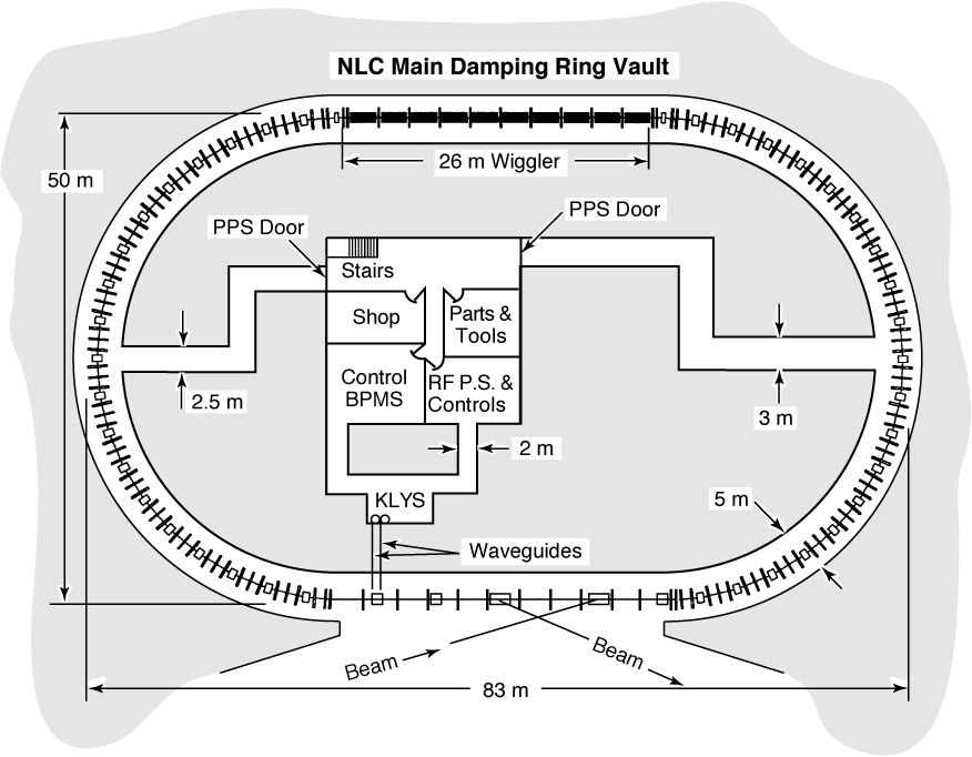
| Figure 2.3: The electron Main Damping Ring (MDR) for the NLC [18]. |
It is the task of the damping rings to produce a beam that is in an optimum condition for acceleration and collision by vastly reducing the transverse beam emittance. This is achieved by making use of the same synchrotron energy loss process described in Section 1.2.3. The electron main damping ring for the NLC is shown in Fig. 2.3. The electron beam is injected into the damping ring and circulated many times: each time it circulates it undergoes the alternate processes of acceleration and energy loss through synchrotron radiation. When the beam passes around either of the two arcs in the damping ring, the curved trajectory causes synchrotron radiation to be emitted, reducing the energy of the electrons. The beam then passes through a series of accelerating cavities which reaccelerate the beam. The emittance reduction occurs because the electrons lose energy in their current direction of travel, but are accelerated only in the longitudinal direction i.e. they lose energy in 3 dimensions and gain energy in 1. This helps to narrow the trajectories of the electrons within the beam until they all lie in approximately the same direction, hence reducing the emittance.
In addition to the energy loss within the two damping ring arcs, a wiggler is used in one of the straight sections to further increase the synchrotron radiation energy loss. A wiggler consists of a series of dipole magnets: the alternating magnetic field, caused by the alternating dipole arrangement within the wiggler, causes the beam to undulate in its trajectory [26]. As the beam undulates it also emits synchrotron radiation in the direction of particle motion, increasing the damping rate per revolution within the damping ring13.
For the NLC, the normalised emittance upon extraction for the damping rings must be reduced to
The bulk of the NLC is made up of the main accelerator tunnel, also referred to as the main linac (see Fig. 1.3). The main linac is used to accelerate the two beams from the post-injector energy of 8 GeV up to the collision energy of 250 GeV (500 GeV for the intended upgrade — see Table 2.1). It is 12.3 km long and consists of 26 sectors, each 468 m long [13]. To reach the intended CMS energy of 500 GeV, only half the linac will be filled with accelerating structures: the other half would be filled for the 1 TeV upgrade. Each sector is split into 9 discrete RF distribution units, each of which contains 8 klystrons and 8 groups of 6 0.9 m accelerating structures [13] — more information on the nature of these structures, and the power delivery systems used to drive them, is given in Section 2.3.
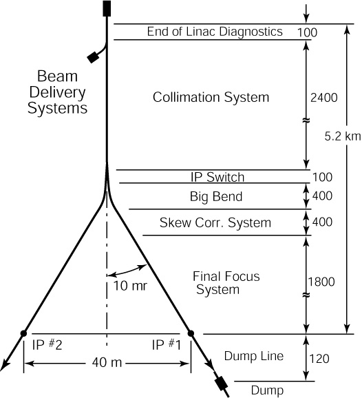
| Figure 2.4: A schematic diagram of the 1996 layout of the NLC beam delivery system [18]; dimensions, except where marked, are given in metres. |
At the end of each of the linacs is the beam delivery system. The purpose of the beam delivery system is to prepare the beams from the linacs, that have now been accelerated to the correct energies, for collision. The role of the beam delivery system is essentially to ensure that the two beams arrive at the IP with the correct spot size. The full NLC beam delivery system consists of a collimation system, the beam switchyard, the final focus, the interaction region (IR) and the beam extraction lines and beam dumps [6]; the beam delivery system is shown in Fig. 2.4.
The first stage of the beam delivery system is the collimation section. The purpose of the collimation system is to remove the proportion of the beam halo that would otherwise interfere with the accelerator or, more importantly, the detector and interaction region (see footnote 2). As such, it has the following requirements [28]:
The collimation system is made up of a series of spoilers and absorbers that are used to ‘scrape off’ the unwanted part of the beam halo (as given by the requirements above). The purpose of the spoiler (or primary absorber) is to ‘blow up’ the beam halo by increasing the angular divergence of the portion of the beam that is intercepted. This prevents the rest of the collimator — the absorber (or secondary absorber) — from having to absorb a large amount of the beam halo, and hence dissipate a large amount of power, within a relatively small amount of material close to the beam [18]. The spoiler is usually much thinner than the absorber — less than a single radiation length, as opposed to
While the whole of the beam delivery system, up to the IP, includes collimation of some kind, the bulk of the collimation system is located upstream of the beam switchyard (BSY). The switchyard is used to direct the bunch train from the linac to one of the two IP's (see Fig. 1.3). Following the switchyard is the final focus system. The purpose of the final focus is to squeeze the beams down to the correct geometry at the IP whilst minimising aberrations introduced in the beam optics by the extremely strong focusing elements (see Section 2.2 for further details). More information on the final focus is given in Section 2.2.5.
The non-zero crossing angle at the IP, of some 20 mrad, means that it is not possible to use the same beamline to deliver the beam to and extract it from the IP: as such, two extraction lines are used to transport the spent beams to the beam dumps. The beam dump is required to dissipate up to 20 MW of spent beam power after the beams have collided at the IP. The beam dumps are situated some 166 m downstream of the IP and consist of a large water tank, interleaved with water-cooled copper plates [18].
In addition to the final focus, the NLC makes use of crab cavities to further enhance the luminosity [29]. Crab cavities are essentially RF cavities with a very fast rise time: as each bunch passes through the cavity, an oscillating transverse electric field kicks the head and tail of the bunch in opposite directions, rotating the bunch and aiming it towards the opposite bunch [30]. The result is that, while the bunches are still subject to a crossing-angle, the collision itself occurs as if the bunches had arrived head-on: this means that each bunch views the opposite bunch as having a smaller horizontal spot size and the luminosity is enhanced.
As mentioned in the previous section, the majority of the collider is made up of long straight accelerator sections that are used to accelerate the beams to the required energies. However, for a successful accelerator, it is not enough to merely accelerate the beam. All accelerators have to achieve the steering and confinement of a charged particle beam along a desired trajectory: colliding 2.7 nm beams from a distance of 32 km is not something that can be achieved without external disturbance or correction. A description of the dynamics of charged particle beams within the confines of the accelerator is now given.
While the charge of the electrons (or positrons) within a beam would naturally cause the beam trajectory to diverge, they also provide a method of constraining the beam to a desired trajectory. The method adopted in accelerators is to use various types of magnets interspersed at regular intervals along the accelerator. When a charged particle enters a magnetic field, the particle experiences a force F, that is related to the magnetic field strength B, the charge on the particle q and the particles velocity v:
| (2.2) |
Therefore, a charged particle within a uniform applied magnetic field will follow a circular trajectory. The centripetal force required to provide the necessary acceleration to bend a particle through such a trajectory is:
| (2.3) |
for a particle of momentum p travelling along a circular trajectory with a radius of curvature ρ. Combining with Eq. (2.2) gives:
| (2.4) |
The quantity Bρ is referred to as the magnetic rigidity and provides information on the required magnet strength and layout for a charged particle with a particular momentum [25]. As such, by manipulating the strength and orientation of an applied magnetic field, it is possible to bend a charged particle through a desired trajectory and steer the beam.
The simplest type of magnet, which operates on just this principle, is the dipole. A dipole magnet is usually constructed from a pair of coils, which are placed parallel to one another (for an example of a dipole magnet used in the SLAC linear collider, see Fig. 5.7). The magnetic field arising from the current flowing in the pair of coils is, for identical coil dimensions and current flow, completely uniform and is perpendicular to the plane of the coils. As such, any charged particle passing between the coils will travel through a curved trajectory, given by Eq. (2.4). The field strength of the dipole is usually integrated along the length of the dipole, giving the total amount of field that a particle will encounter, and is given in units of
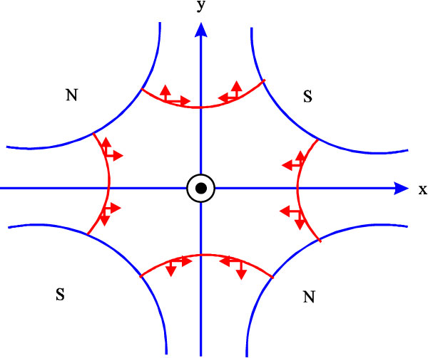
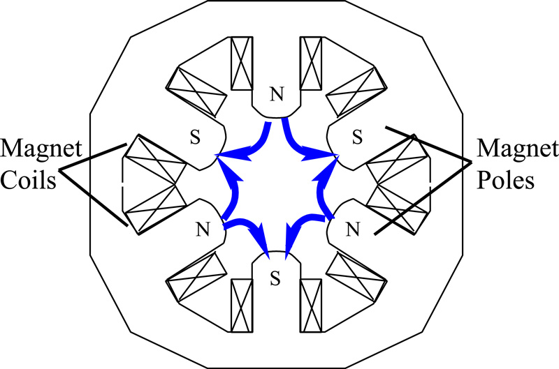
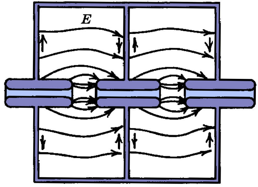
| Figure 2.5: The magnet pole arrangement for a quadrupole magnet [25]. The blue lines mark the magnet poles (polarity indicated as ‘North’ or ‘South’); the red lines mark the magnetic field lines. The red arrows indicate the force applied to a positively-charged particle beam travelling out of the page: the magnet focuses in x and defocuses in y and is therefore defined as a focusing quadrupole. |
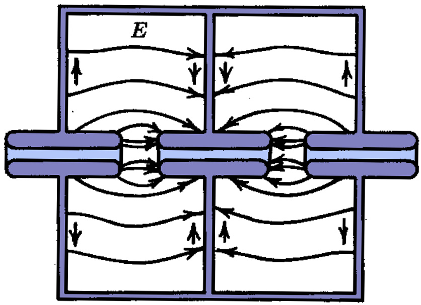
The field produced by a dipole (or series of dipoles), however, will not provide the necessary focusing required to keep a particle beam constrained to a desired orbit. In order to prevent the beam from diverging from this desired orbit, extra focusing is required that will force off-axis particles back onto the desired trajectory: this is achieved with the quadrupole. A quadrupole magnet is constructed from four poles — two ‘North’ and two ‘South’ — which are arranged as shown in Fig. 2.5. By arranging the poles in this manner, the magnetic field increases as a function of the distance from the centre of the magnet, where:
| (2.5) |
For most quadrupoles the horizontal and vertical focusing strengths are of equal magnitude. A quadrupole is usually characterised by the gradient of the quadrupole field, K = dBx/dy = dBy/dx: this quantity is constant and has units of Kilo-Gauss per metre (kGm-1) or Tesla per metre (Tm-1). The magnet strength can also be expressed in terms of the normalised gradient, k, where k = K/Bρ and has units of m-2. As such, this gives rise to a dipole field that varies with distance from the centre of the magnet. The result is that particles that are further off-axis are steered more strongly back towards the centre of the beampipe, giving an overall focusing effect [25].
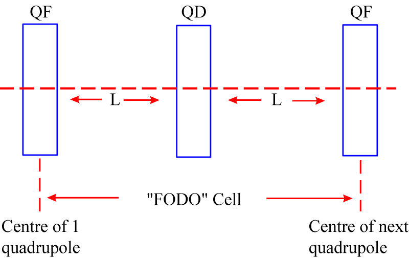
| Figure 2.6: The quadrupole arrangement used to construct a FODO cell (adapted from [25]): alternate focusing and defocusing quadrupoles are separated by drift spaces. |
However, due to the arrangement of the field within the magnet, a quadrupole can only focus the beam in one transverse plane at a time: in the other plane, the beam is actually steered away from the ideal trajectory and becomes defocused. A quadrupole that is oriented such that it focuses in x (and defocuses in y) is referred to as a focusing quadrupole, QF, while a quadrupole that focuses in y (and defocuses in x) is referred to as a defocusing quadrupole, QD. To accommodate for the defocusing behaviour of the magnet, quadrupoles are arranged in pairs, as depicted in Fig. 2.6: this magnet arrangement alternately focuses and defocuses the beam and is called a FODO cell (for FOcusing and DefOcusing).
Accelerators are made up of these FODO cells or something similar but more complex. The arrangement of these magnets, and the effect they have on the beam, is similar to the focusing and defocusing effect of lenses in optics: in fact, the treatment of beams within accelerators is similar to that in geometric optics; more information is given in Section 2.2.3. The result of organising the quadrupoles into such a FODO lattice is to cause the beam trajectories to oscillate around the ideal trajectory (usually the magnetic centre of the accelerator beamline components). These oscillations are referred to as betatron oscillations and are a well-defined function of the spacing and focusing strength of the quadrupoles [31]; more detail is given in the next section. These betatron oscillations confine the particles within the beam to a desired range of trajectories by focusing particles more strongly as they stray further from the ideal orbit.
As mentioned in the previous section, betatron oscillations arise as a result of the FODO lattice arrangement within an accelerator. These transverse oscillations are periodic and follow the standard laws for simple harmonic motion. For oscillations within a FODO lattice, of magnitude x, the general equation (known as Hill's equation) for transverse motion within an accelerator is:
| (2.6) |
where s is the longitudinal distance along the accelerator and K(s) is the restoring force due to the quadrupoles; this restoring force is a function of longitudinal position [25]. It can be shown that solutions of this equation for transverse motion within an accelerator have the form:
| (2.7) |
where εx is the horizontal beam emittance, as defined in Section 2.1.2; φx is the initial phase and is also constant [32]. The two remaining quantities, &betax(s) and ψx(s), are both functions of longitudinal position: &beta(s) is the beta function and describes the amplitude modulation of the transverse beam motion; ψ(s) is the phase advance and describes the change in beta phase; both are dependent on the focusing strength of the quadrupoles [31]. There is a second, identical equation for vertical motion: this is assumed in all the following equations and only the version for x is given. The phase advance is related to the beta function by:
| (2.8) |
As such, the rate of change of transverse position, i.e. the angle, x′, is given by:
| (2.9) |
where
| &epsilon = γ(s)x(s)2 + 2α(s)x(s)x′(s) + β(s)x′(s)2 | (2.10) |
where γ(s) = 1+α2/β [32]. This quantity is invariant under a change of s and, therefore, the beam emittance is a fixed quantity for any periodic accelerator lattice. It is also necessary to define the relative phase advance, μ, where μ(Δs) = Δψ(s). The functions α(s), β(s), μ(Δs) and γ(s) are known as Twiss parameters: there are two of each function — one for each transverse plane — and they are used to characterise the accelerator lattice [31].
In order to construct the quantities described in the previous section, a matrix approach is adopted. While the two beta functions — βx and βy — are continuously varying functions of s, the accelerator itself is not: it is constructed from a number of distinct units e.g. a drift section, a quadrupole, a dipole and so on. As such, it is possible to calculate the various Twiss parameters by using a series of matrices to describe each of the discrete elements from which the accelerator is constructed. For the two horizontal beam parameters, x and x′, the translation between two points along the accelerator, s1 and s2, is given by the following matrix equation:
| (2.11) |
where the subscripts indicate the various parameters at the two points along the beamline [32]. In practice, a 6×6 matrix, referred to as the R matrix, is used:
| (2.12) |
where, in addition to the four transverse beam parameters, l is the longitudinal particle location along the length of a bunch and δ is the relative momentum deviation from the reference particle [33]. For the majority of accelerator components there is no x-y coupling and, if all components are symmetrical about y = 0, the R-matrix reduces to:
| (2.13) |
In order to describe beam motion along the accelerator, a matrix is used to describe each of the beamline components: for example, using just the two transverse beam parameters x and x′, the R-matrix for a drift space is:
| (2.14) |
for a drift space of length L, and the corresponding matrix for a quadrupole magnet is:
| (2.15) |
where l is the length of the quadrupole and k the normalised gradient, as given in Section 2.2.1 [34]. For a thin lens approximation, where
| (2.16) |
where
| (2.17) |
with the usual rules for matrix multiplication followed and the numbers indicating the order in which the elements are encountered between s1 and s6. As such, it is possible to track the motion of the beam through the accelerator, given the initial beam conditions. This matrix approach can also be used to track the evolution of the shape of the beam emittance ellipse (as shown in Fig. 2.2).
The equations given in the previous section allow the motion of ideal particles to be predicted exactly. However, not all particles within a bunch will behave in this well-defined manner: errors in the energy or momentum of individual particles, as opposed to the position/angle error that the FODO lattice is designed to counteract, can also lead to significant beam losses. Errors arise in the particle energy/momentum as a result of many effects, such as scattering from gas molecules during the acceleration process or the emission of synchrotron radiation, as well as any energy error introduced at injection. This results in a spread in the momentum of the particles within a beam, Δp/p.
The result of such a momentum error is that the magnetic rigidity, Bρ, changes, in accordance with Eq. (2.4), and hence the bending radius of any dipole magnet; this effect is called Dispersion [25]. As such, in regions of non-zero dispersion a beam will experience an increase in transverse beam size due to the momentum spread in the beam, as a result of the momentum dependence of Bρ. The transverse displacement, Δx, due to the momentum spread is given by:
| (2.18) |
where D(s) is called the Dispersion function. This dispersion function can be calculated from the lattice in the same way as the beta functions and is computed independently for x and y.
In addition to the dispersion, the momentum spread also causes a change in the focusing strength, and hence the focal length, of the quadrupoles, as a result of the change in magnetic rigidity: this effect is referred to as Chromaticity, ξ. The chromaticity is defined as the relative change in phase advance that results from the momentum spread:
| (2.19) |
As before, there is a horizontal chromaticity, ξx, and a vertical chromaticity, ξy. Correction of the chromaticity (called chromatic correction) is important, particularly at the IP, where the beta functions become very small (denoted by β* in Table 2.1) and the final doublet (see below) attempts to focus the beam to a point. As a result of the momentum-dependent variation in focal length, a lack of such chromatic correction at the NLC would result in an increase in spot size by two orders of magnitude [6].
| Figure 2.7: The layout of a sextupole magnet (adapted from [34]). The magnetic field lines are shown in blue, with the polarity of the 6 magnet poles indicated; the 12 magnet coils are also marked. |
Correction of the chromaticity is achieved with another, higher-order magnet, called a sextupole. As its name would suggest, the sextupole has 6 magnet poles of alternating polarity: the magnet pole arrangement and resultant B-field can be seen in Fig. 2.7. This pole arrangement gives the following B-field [35]:
| (2.20) |
This means that a particle that passes through the sextupole receives a deflection that is proportional to the square of the horizontal distance from the centre of the sextupole. As such, it behaves like a quadrupole whose focal length is a function of the horizontal distance from the centre15. By placing the sextupole next to a quadrupole in a region of finite dispersion, the transverse beam spread that results from such a dispersive region (see above) allows the sextupole to correct for the chromaticity of the quadrupole. For a quadrupole/sextupole pair, the beam deflection is given by:
| (2.21) |
where Kq is the integrated field strength of the quadrupole, Ks is the integrated field strength of the sextupole, ls is the length of the sextupole, Dx is the horizontal dispersion and δ is the relative momentum error, Δp/p [36]. It is therefore possible, by introducing dispersion in only one plane (the horizontal), to correct for the chromaticity in both planes. In addition to the desired correction, a sextupole will also introduce unwanted nonlinear effects: cancellation of these higher-order terms is covered briefly in the next section.
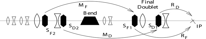
| Figure 2.8: A schematic diagram of the magnet layout for the chromatic correction section of the NLC Final Focus optics: the quadrupoles are indicated by the lenses (for focusing/defocusing quads), with the sextupoles marked by hexagons. MF,D indicates the transport matrices for sextupole pairs and RF,D the transport matrices to the IP [37]. |
As mentioned in the previous section, chromaticity correction is most important in the final focus section of the beam delivery system (see Section 2.1.3 for details of the complete beam delivery system). The purpose of the final focus is to reduce the beam spot size at the IP to provide the maximum luminosity [29]. This is achieved with a pair of very strongly focusing quadrupoles — one for x and one for y — that are situated close to the IP: these are usually referred to as the Final Doublet (FD). The innermost quadrupole of the final doublet is mounted 4.3 m away from the IP (a distance denoted by L*): the full layout of the NLC final focus is shown in Fig. 2.8.
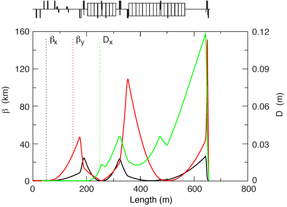
| Figure 2.9: The horizontal and vertical beta functions (βx, βy) and horizontal dispersion (Dx) for the full NLC Final Focus optics; the magnet layout shown in Fig. 2.8, including the IP, are at the right hand end, at ~650 m [13]. |
The corresponding beta functions for the final focus are shown in Fig. 2.9. The major source of chromaticity at the IP is the two final doublet quads: as such, most of the final focus is geared towards the cancellation of this chromaticity [13]. A pair of quadrupoles is required to focus in both planes and demagnify the beam to a waist at the IP. In order to locally cancel the chromaticity produced by these very strongly focusing magnets, a pair of sextupoles — one for x and one, rotated by 180°, for y — is placed upstream of each of the final doublet quads to apply the necessary chromatic correction. A dipole is then used to create horizontal dispersion in the beam to provide the necessary beam spread for the sextupole correction (see above). In addition, the sextupoles themselves generate higher order geometric abberations: to help cancel these unwanted terms, a second pair of sextupoles is located upstream of the first pair, separated by 180° of beta phase [37]. This arrangement of sextupoles is referred to as the chromatic correction section [29].
The front end of the final focus is referred to as the beta-matching section. The purpose of the beta-matching section, as the name would suggest, is to match the beta functions at the end of the linac to those required by the final focus. In other words, one tracks back from the final doublet, through the chromatic correction sections, tracking the beta functions and phases and attempts to match the beta functions at the start of the chromatic correction section with those that arise at the end of the collimation section (see Fig. 2.4). This is the purpose of the 4 quads situated furthest upstream in Fig. 2.9.
The acceleration of charged particles is in essence relatively simple. In an electric circuit, an electric current in a medium, consisting of a continuous flow of electrons, is created with the application of a potential difference, or voltage. The application of this potential difference gives rise to an electric field within the medium that pulls the electrons along, creating the current.
An almost identical principle is adopted for the acceleration of charged particles within an accelerator. Instead of transporting the electrons (or positrons) through a current-carrying medium, the particles are confined to a beampipe, using the principles described in Section 2.2. However, the key difference is in the application of the accelerating potential. It is no longer possible to apply a static, DC potential between two points to accelerate the electrons (the ‘Van De Graaff’ accelerator), since it is impossible to sustain the enormous E-fields required: an accelerating gradient of many MegaVolts per metre (MVm−1) is necessary to reach the required GeV energies [38]. Instead, time-varying fields are used to accelerate a bunched beam.
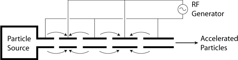
It may seem at first glance that using an AC potential to accelerate particles would be completely counterproductive, producing no net accelerating gradient. However, it is the very fact that the time-integrated E-field is zero that allows such high fields, of many MVm−1, to be sustained. The simplest way to apply such a varying potential is the Wideroe scheme, shown in Fig. 2.10.
| Figure 2.10: The Wideroe scheme for charged particle acceleration (adapted from [38]). A time-varying voltage is applied to alternate plates, accelerating the particles between the drift tubes; the voltage is indicated by the arrows. |
The beampipe is divided into sections, with a gap between each: an alternating voltage is applied to the plates in the manner indicated in Fig. 2.10. The applied voltage is at its maximum when the particles reach the gap between these drift tube sections and is zero when the particles are right in the centre of a drift tube. This means that, with the particles in between drift tubes, the previous section repels the particles forward, with the approaching section also attracting the particles forward. This method also has the effect of causing the particles to bunch, since slower (or lower energy) particles will be lost from the back of the bunch, while faster particles will not receive the maximum acceleration and will therefore also move backwards into the bulk of the bunch.
However, the disadvantage of such a scheme is that there is no way to drive lower energy particles with a higher voltage while driving higher energy particles with a lower voltage to longitudinally compress the bunch. In addition, power is radiated from the drift tubes since there is no way of preventing it from being lost, reducing the efficiency of the accelerator. The bunch also only receives a brief acceleration between beampipe sections. The solution to the first two problems is to fully enclose the accelerating gap between the beampipe drift sections in a resonant cavity. The primary benefit is that the energy produced by the voltage source is trapped within the cavity and dissipates only slowly into the walls of the cavity [38].
|
|
|||
| (a) π mode | (b) 2π mode | |||
| Figure 2.11: The π and 2π modes for adjacent single-gap cavities [39]. The width of each cavity is governed by the frequency of the injected RF and the mode utilised; the mode number indicates the phase difference between adjacent cavities. | ||||
Instead of applying a voltage externally to the structure to provide the necessary gradient, the E-field is injected directly into the structure in the form of high frequency RF. The intention is then to make sure that the E-field within the cavities sets up a resonant oscillation: as such, the cavity length is usually designed to be half the wavelength of the injected RF, λ, where
There are two possible modes in which to inject the RF, referred to as the π mode and the 2π mode, both of which are shown in Fig. 2.11. In the π mode (Fig. 2.11(a)) each cavity is out of phase with the adjacent one, whereas in the 2π mode (or 0 mode: Fig. 2.11(b)) each cavity is in phase. This means that, in the 2π mode, the radial walls of the cavity become redundant and it is possible to immerse the whole structure in a single E-field: this is known as an Alvarez linac [38]. For a particular frequency, the π mode allows for a gradient twice as high as the 2π mode and therefore a shorter linac [39].
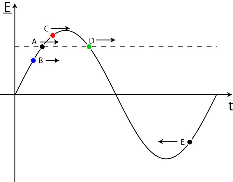
| Figure 2.12: The accelerating gradient, in the form of the applied E-field, experienced by 5 different particles in an accelerating cavity as a function of the time at which they arrive at the cavity t (adapted from [25]). A is the synchronous particle, B is higher energy, C is lower energy, D is on the edge of stability and E experiences a retarding potential. |
By appropriately selecting the phase (i.e. the timing) of the E-field introduced into the cavity, it is possible to significantly compress the bunches and correct for any longitudinal position or energy error: this is shown in Fig. 2.12. While it may seem that the maximum acceleration is gained by introducing the electron bunch into the cavity in phase with the maximum E-field strength, it is actually more advantageous to introduce the bunch slightly early (particle A). By doing so, any particle that arrives slightly earlier (usually as a result of being slightly too high in energy) will experience a smaller E-field and accelerating force (particle B). Conversely, any particle arriving later (with too low an energy) will receive a greater acceleration (particle C).
This gradient in the energy gain causes the particles to bunch together at the frequency at which the RF is applied (which is often referred to as the bunching frequency) — this clumping region in the RF is called an RF bucket. This includes particles that are very far off in energy: those that arrive much later will receive a negative acceleration (particle E) and be slightly retarded, forcing them back into the bunch behind. They then proceed to undergo the same under-acceleration/over-acceleration process as described above.
|
Figure 2.13: The longitudinal phase space ellipse, in |
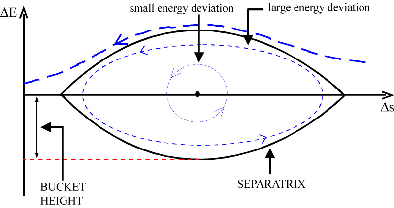
As such, the off-energy particles within a bunch actually circle around the central particle (particle A in Fig. 2.12, referred to as the synchronous particle) in energy-position space, forming another phase-space ellipse: as with horizontal and vertical phase space (cf. Section 2.1.2 and Fig. 2.2), the area of this ellipse is referred to as the longitudinal emittance. The boundary of this phase space ellipse is called the separatrix and marks the stable boundary of the particles within a single bunch (particle D in Fig. 2.12): this is shown in Fig. 2.13. The particles within the separatrix undergo the cyclical relative acceleration/deceleration: those outside the separatrix are lost, either to the following bunch or from the accelerator altogether. In this way, particle motion with longitudinal stability and a small energy spread is achieved.
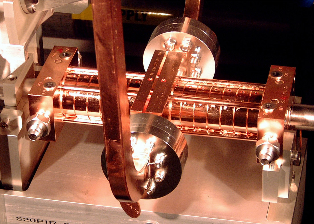
Modern accelerating structures operate on principles similar to those described in Section 2.3.1. However, since electrons of a few hundred MeV are already highly relativistic, it is not necessary to vary the length of the drift spaces within a structure as is usually done with an Alvarez structure. As such, it is possible to shorten the drift spaces a great deal so that the electron bunches spend more time within the accelerating field. Such a structure is called a Standing Wave structure: an example of a standing wave structure for the NLC is shown in Fig. 2.14 [38].
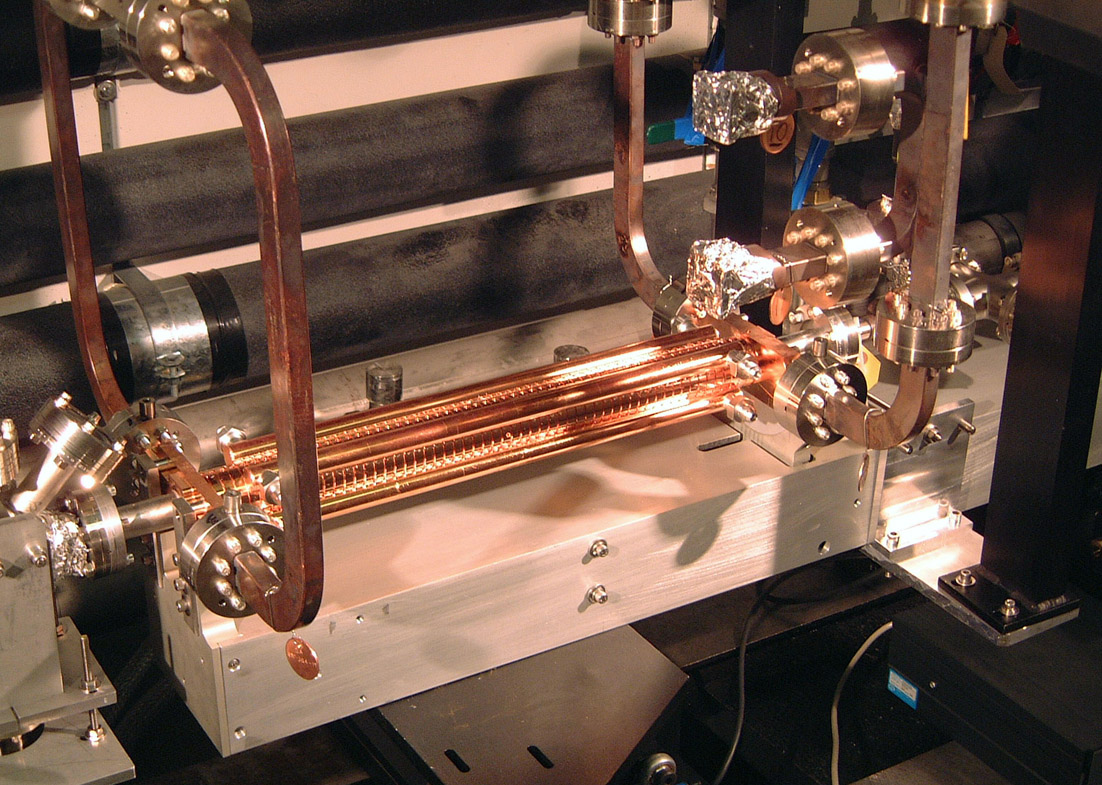
| Figure 2.14: A 15-cell NLC copper standing wave structure, installed at the NLCTA (see Section 5.1 for details of the NLCTA) [40]. The two waveguides feed the RF power into the structure through the centrally-mounted input couplers. |
The RF is introduced into the structure in such a way (i.e. with the correct mode) that a standing wave is set up along the length of the structure, with nodes at the interfaces between the cavities, or cells. The standing wave consists of a longitudinal electric field, with no longitudinal magnetic field (a transverse magnetic, or TMmn mode): this provides the necessary accelerating force in the form of the longitudinal E-field. Such a structure is usually driven in the π mode, with the E-field configuration shown in Fig. 2.11(a) [39]: the size of the cells is designed to be resonant at the accelerating frequency. The structure uses a single pair of centrally-mounted RF input couplers to deliver power into the structure (see Fig. 2.14). This input power is used to sustain the accelerating field within the structure and deposit power to the beam: any unused power either gets absorbed by the structure (hence the copper cooling pipes mounted on the outside of the structure) or escapes down the beampipe.
| Figure 2.15: An NLC travelling wave structure, installed at the NLCTA [40]. The structure has 4 RF couplers: two input and two output. |
A development of the standing wave structure, used almost exclusively in linear accelerators, is the Travelling Wave structure: an NLC travelling wave structure is shown in Fig. 2.15. The method of acceleration is similar to the standing wave structure, in that a time-varying longitudinal E-field is used to accelerate the beam as it passes through the cavity: however, instead of setting up a fixed standing wave (forming nodes of oscillation at the cell boundaries and antinodes in the centre of each cell), the sinusoidal E-field is now launched from the front of the structure and runs along in synchronisation with the beam [39]. As such, the maxima and minima of the accelerating field are no longer fixed (‘standing’) but move with the beam (‘travel’), providing a continuous acceleration.
Instead of behaving as a resonant cavity, the structure now behaves as a waveguide, allowing RF power to travel along its length [38]. Waveguides are essentially tubes, with either a rectangular or circular cross section, that allow the transmission of electromagnetic waves (and hence RF power) with virtually no power loss. The energy is stored and transmitted in the form of resonant electric and magnetic fields within the structure [39]. The available modes of oscillation within the waveguide, for a particular frequency, are fixed by the transverse dimensions of the waveguide: the minimum frequency sustainable within a waveguide is referred to as the cutoff frequency [41].
There are two main types of oscillation: the TEmn, or Transverse Electric modes, where there is no longitudinal E-field, and the TMmn, or Transverse Magnetic modes, which has no longitudinal B-field. In addition, there are also TEM modes with purely transverse fields. The subscript mn indicates the order of the mode, with higher order modes requiring larger resonant cavities16. Clearly, for the purposes of acceleration, a longitudinal E-field is required to accelerate the beam along the beampipe: as such, only TM modes are used within the structure [39]. The RF is injected into the structure at the front and extracted at the rear, hence the doubling of the number of waveguide couplers seen in Fig. 2.15.
The rate of advance of the E-field maxima (the phase velocity, vp) is set by the spacing of the cavities within the structure and should be the same as the particle velocity
In general, travelling wave structures are cheaper to produce for a particular gradient: however, it is possible to achieve higher gradients with a standing wave structure [13,42]. Travelling wave structures are necessarily longer, since it is desirable to use up all the injected RF as it is dissipated along the length of the structure before being extracted. A standing wave structure has no such condition, since all the power is retained within the structure. As such, the shorter standing wave structures can hold a higher gradient: in addition, any breakdown within the cavity will result in a higher power deposition in a travelling wave structure, since the longer structure holds more power [43].
However, both cavity types are required to achieve a higher gradient than is actually needed. This is a result of a phenomenon called beam loading. Beam loading results from the interaction of the beam with the conductive walls of the accelerating structure. As the beam passes through the cavity, the EM-field surrounding the beam interacts with the cavity, producing a wakefield that acts against the accelerating field: this reduces the magnitude of the longitudinal E-field and hence the accelerating gradient. This is similar to the back-EMF produced by an electric motor as a result of its inductance. This gradient reduction occurs gradually along the length of the bunch train, resulting in a smaller gradient for the rear bunches. To compensate for this effect, the RF input power at the NLC is ramped, so that the power reduction that occurs as a result of beam loading matches the power increase supplied by the RF system. As a result, the NLC accelerating structures are required to achieve an unloaded gradient of 70 MV/m, but a loaded gradient of 55 MV/m [13].
Since the size of the cavities, in all dimensions, is dependent upon the RF frequency, higher frequency RF drive is favourable as it provides both a higher gradient and shorter bunches (see Section 2.3.2) for a smaller, cheaper structure: however, higher frequency RF is more difficult (and more expensive) to produce, with correspondingly tighter tolerances required in the manufacture of the structures, further increasing the cost; there is therefore a tradeoff in achieving the cheapest and most beneficial solution. The NLC main linac uses an X-band drive frequency of 11.424 GHz, with copper travelling wave structures [13].
| Figure 2.16: A schematic drawing of an NLC X5011 periodic permanent magnet (PPM) focusing klystron [18]. The drift tube consists of a number of small RF cavities; the ion pumps are required to prevent the electron beam scattering off gas inside the klystron. |
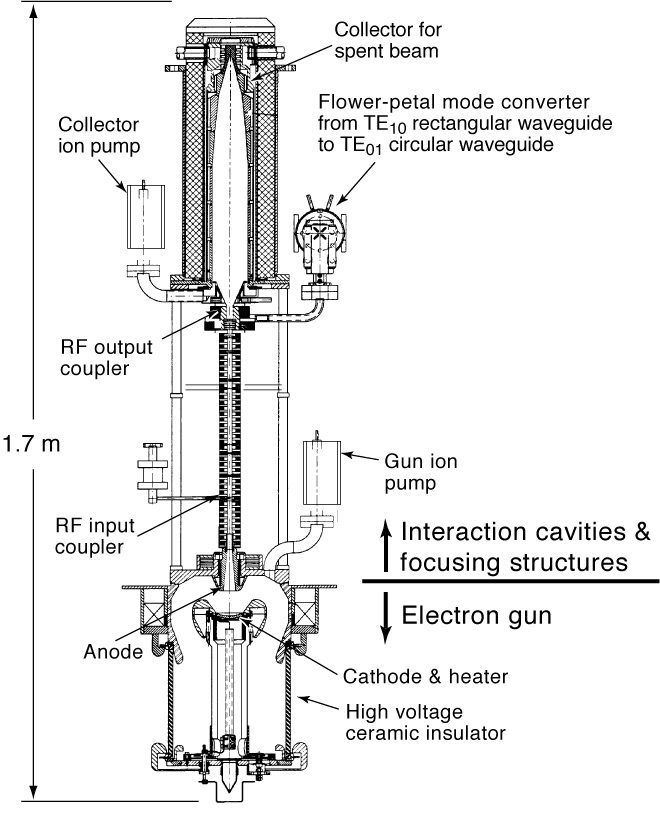
Given the enormous gradients that have to be sustained within the NLC accelerating structures, a correspondingly large amount of power is required to sustain these large E-fields. As such, the delivery of RF power to the structures is a crucial part of the NLC main linac. In order to produce the 50 MW peak powers required by the RF system, a high power RF source called a klystron is used. A schematic diagram of an NLC klystron is shown in Fig. 2.16.
A klystron is almost an accelerator in miniature. An electron gun at the bottom of the klystron creates a burst of electrons. This electron pulse then passes through a resonant bunching cavity: into this cavity is injected a steady RF flow (CW, or Continuous Wave) at the desired accelerating frequency. Since the cavity is also resonant at this frequency, the electron beam becomes strongly bunched at this frequency as it travels out of the cavity. The bunched beam then passes through a second, output cavity that is also resonant at the accelerating frequency. This resonance causes the bunched electron beam to very strongly excite the cavity at the accelerating frequency: the RF produced within the cavity as a result is then coupled out through a waveguide, which carries the amplified RF power out to the structures (see above). The electron beam is then dumped into a beam stop at the top of the klystron [44].
In practice, a number of input and output cavities may be used to maximise both the electron bunching and the amount of RF power that can be extracted from a single klystron. This use of resonant cavities creates a large amplification of the RF signal input to the bunching cavity: gains of 106 are possible with modern pulsed-power klystrons [44]. Two power sources are required to provide the input power to the klystron. The RF input to the bunching cavity is produced by a low-level RF system: this provides the RF ‘input’ signal that is amplified by the klystron and is usually a CW microwave source, such as a travelling wave tube (TWT) [13].
The input power to the klystron is provided, through the electron gun, by a modulator [45]. A modulator is used to produce the pulses that drive the electron gun in the klystron and produce the high intensity electron beam. It is through the modulator pulse that the klystron receives the power that amplifies the low level RF input into a high power output to drive the structures. The modulator pulse is a DC square pulse that lasts for a few microseconds: pulsing the modulator allows for a higher peak output and therefore larger power delivery to the accelerating structures.
The klystrons in the NLC are assembled into groups of 8, referred to as an ‘8-pack’, with each powered by a single 500 kV modulator: these make up a single RF distribution unit, of which there are 9 in each linac sector (see Section 2.1.3). Each klystron 8-pack supplies 8 groups of 6 structures, with power delivered to each group of structures via a pulse compression system called the Delay Line Distribution System (DLDS) [13]. DLDS allows the combination of the 3.2 µs RF pulses produced by each klystron into 8 consecutive 396 ns pulses, which are then delivered to the groups of 6 structures. As such, up to 600 MW of peak power can be delivered to the accelerating structures [13].
The IP is the most important part of the entire accelerator. It is the point at which the electron and positron beams are brought into collision and around which is mounted the detector to measure the decay products resulting from these collisions. The beam-beam interaction in linear colliders is markedly different from that in synchrotron machines, primarily as a result of the extreme beam geometry used in linear colliders. From Section 2.1.2, the luminosity is defined as:
|
with the quantities as defined previously. As one would expect, the collision rate is a function of the temporal and spatial density of the particles brought into collision i.e. the number of particles forced into collision per second (indicated by nN2f) and the transverse size of the beam bunches (governed by the r.m.s. transverse beam sizes at the IP, σx* and σy*).
To counteract the lower bunch crossing frequency, a linear collider uses a considerably smaller beam spot size than a synchrotron. However, this in turn introduces other effects into the beam-beam interaction which do not affect collisions in a synchrotron. Whereas a synchrotron will recycle the beams continuously for minutes or hours at a time, with virtually no ill effects from each bunch crossing, the violence of the beam-beam interaction in a linear collider is considerable: the carefully prepared bunches are virtually torn to pieces by the intensity of the collision. These beam-beam effects can essentially be split into two categories [46]:
The phenomenon of beamstrahlung is closely related to two other well-known phenomena: bremsstrahlung and synchrotron radiation. Both processes involve photon emission by accelerated charged particles. A description of synchrotron radiation is given in Section 1.2.3. Bremsstrahlung, or braking radiation, is the emission of a single photon by a charged particle as it traverses a bulk material and passes through the EM-field surrounding an atom. It is most commonly seen in electromagnetic showers as part of the energy loss process of an energetic particle in a scintillator or absorber.
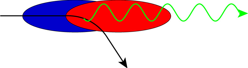
| Figure 2.17: Schematic representation of beamstrahlung emission during the beam-beam collision (adapted from [47]). The trajectory of a single particle in the electron bunch (blue) is indicated by the curved black line: passing through the EM-field of the colliding positron bunch (red) causes it to bend and emit a beamstrahlung photon (green). |
The emission of beamstrahlung occurs not in an absorbing medium, but in the EM-field of a charged bunch. As the two oppositely charged bunches pass through one another, the EM-fields surrounding each bunch cause the trajectories of the particles within the opposing bunch to bend, stimulating the emission of energetic photons: this is illustrated schematically in Fig. 2.17. For bunch dimensions of the NLC, the average EM-field in each bunch during collision is in the kilo-Tesla range [46]: with such large fields, the energy and luminosity loss at the IP can be significant. Not only can beamstrahlung increase the energy spread within the beam, in the same manner as ISR18, but the beamstrahlung photons can also pair produce and cause scattering collisions within the bunch [36]. In addition, if not adequately minimised, energy loss by beamstrahlung can impose an upper limit on the possible CMS collision energies.
The beamstrahlung phenomenon is characterised by the beamstrahlung parameter, Υ, which is a measure of the field seen by a beam particle in its rest frame and is defined as follows [48]:
| (2.22) |
where me is the electron/positron rest mass, q is the electron charge, pμ is the electron four-momentum and Fμν is the mean energy-momentum tensor of the bunch field. The critical magnetic field, Bc, is defined as:
| (2.23) |
giving a mean bunch field for the NLC of ⟨E + B⟩ ≈ 990 Tesla (using the parameters from Table 2.1). During a single collision, the field strength will vary along the length of each bunch. It is possible to define an average and maximum beamstrahlung parameter — for beams with a Gaussian transverse particle density, these are [46]:
| (2.24) |
where re is the classical electron radius, α is the fine structure constant and σz* is the IP r.m.s. bunch length. The two key parameters resulting from beamstrahlung are related to the photon energy loss. The average number of photons radiated during a single bunch collision per electron, nγ, is given by [48]:
| (2.25) |
where λc is the Compton electron wavelength and Υ = Υave. To retain a usable energy spectrum at the IP, nγ should be limited to a value around one [36]. It is also necessary to minimise the amount of energy radiated through beamstrahlung per bunch crossing for the reasons given above. The fractional beamstrahlung energy loss per bunch, δB, is given by [48]:
|
2 |
(2.26) |
with Υ = Υave. Along with the beam size dependence of the beam-beam disruption (see Section 2.4.2 below), it is this dependence of Υ on
In contrast to the quantum nature of beamstrahlung, disruption describes the effect of the classical electromagnetic field surrounding each bunch during the collision and the resulting change in beam trajectories [48]. While the interaction of two charged bunches is a highly complex process, it can be simplified somewhat by making the following assumptions [46]:
For a single particle within a bunch, the equation of motion during collision is given by [46]:
| (2.27) |
with a similar equation for x; here, N is the number of particles in the opposing bunch, nL is the longitudinal bunch density and Φ is the electrostatic potential. Near to the centre of a bunch with a Gaussian transverse particle distribution i.e. where
| (2.28) |
Substituting this expression for Ψ into Eq. (2.27) gives:
| (2.29) |
where y is the transverse beam separation. Assuming that the collisions are approximately head-on
| (2.30) | |||||||||||||||||||||||||
where y0 is the mean bunch separation and
| (2.31) |
The disruption parameter is therefore the ratio of the r.m.s. bunch length to the ‘focal length’ of the bunch. Due to the difference in transverse beam dimensions there is a disruption parameter for each transverse dimension: since the vertical beam spread is much the smaller (and therefore dominant) in linear colliders, Dy is normally quoted. For a uniform longitudinal particle distribution, substituting Eq. (2.31) into Eq. (2.29) gives:
| (2.32) |
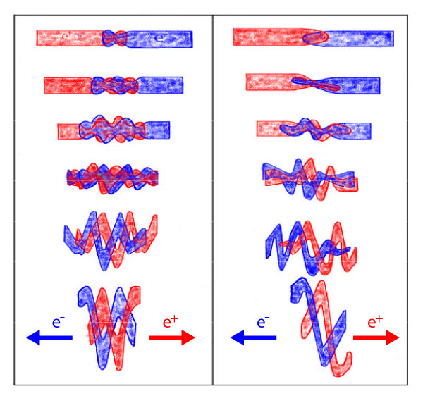
during the time that the two bunches are coincident [46]. This equation has solutions of the form sinAt and cosAt, giving rise to sinusoidal oscillations. This essentially means that, as the two bunches pass through one another during collision, they oscillate across one another: this is illustrated in Fig. 2.18. This figure shows the effect of
| Figure 2.18: The effect of the beam-beam interaction on two colliding bunches for D = 40 at discrete time intervals during collision [50]. The left series shows a head-on collision, with the right series showing a slight vertical offset between the two bunches; illustrations are highly schematic. |
The effect of disruption is twofold [49]. Firstly, the mutual attraction of the two bunches causes their trajectories to curve, as given by Eq. (2.30). This curvature, coupled with the oscillations described above and the waist that occurs at the IP, causes a large increase in the angular divergence of the beam as it exits the collision region. Special care must therefore be taken in transporting the beams from the IP to the beam dumps. Secondly, disruption can actually cause an increase in the luminosity, due to the mutual attraction of the two beams: this is particularly effective for a relatively small beam-beam offset, as the attractive force pulls the two beams together upon collision. These are described in more detail in the next section.
Due to the large focusing strength of the final doublet quads, the beam is focused to a very narrow waist at the IP, with
| (2.33) |
The divergence parameter gives a measure of the natural divergence of the beam at the IP (i.e. the IP emittance, εx,y* [48]: a smaller β* results in a larger IP beam divergence due to the focusing force applied to the beam, while a smaller bunch length σz can counteract this divergence by reducing the longitudinal space in which the two bunches interact.
In addition to the hourglass effect, the two colliding beams also undergo a slight compression at the IP as a result of their mutual attraction. This is called the Pinch effect and causes an enhancement in the luminosity, since the beam spot size is reduced by this IP compression. The pinch enhancement factor, HD, gives a measure of the luminosity gain as a result of the pinch effect and is defined as:
| (2.34) |
where L is the measured luminosity and L0 is the nominal luminosity without the pinch enhancement [46]. Due to the complex nature of the beam-beam interaction, there is no precise method of calculating HD; however, it can be approximated by [49]:
| (2.35) |
where only the vertical disruption and divergence parameters are used, since the beam is much smaller in the vertical direction and therefore has much greater vertical disruption. The dependence of HD on Dy is due to the condition of the beams at collision: with a small disruption the beam sees a slight enhancement, increasing the luminosity, as a result of the focusing effect of the beam-beam interaction; with too high a disruption, however, the bunches rapidly fall apart and the luminosity falls off. Determining HD with any degree of precision is only possible with computer simulations [46].
The final effect that results from beam disruption is that of beam-beam deflection. Since the beams are mutually attractive, they will be pulled towards each other when their EM-fields coincide. If the two bunches have a net transverse offset, this attraction will cause the beams to bend round one another, resulting in the curvature of the beam trajectory at the IP.
The deflection curve resulting from this beam-beam kick is essentially a macroscopic version of the force exerted on a single particle from the E-field of the opposite bunch, as described in the previous section (see Section 2.4.2). As such, the outgoing angular distributions are dependent to some extent on the disruption, with the deflection parameter defined as [46]:
| (2.36) |
The outgoing beam deflection angle has the following approximate dependence on ΘD [48]:
| (2.37) |
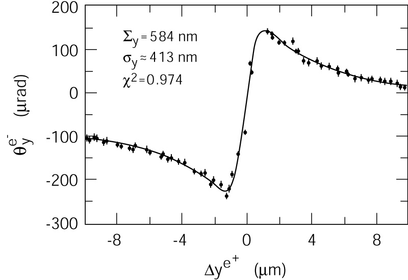
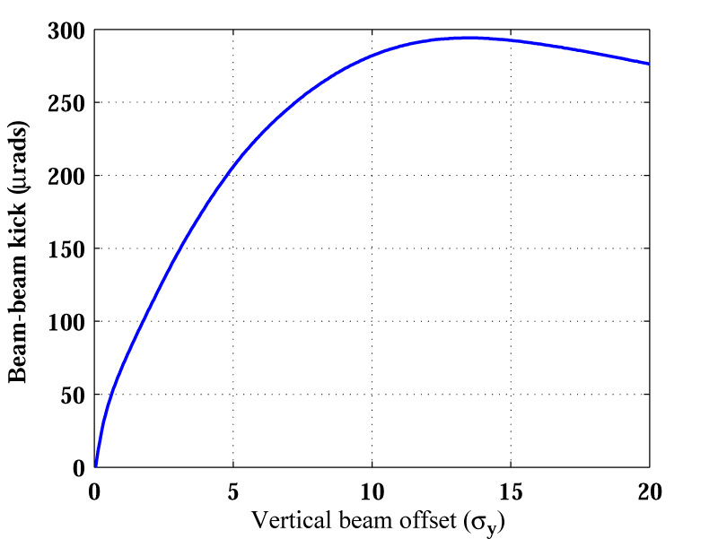
This phenomenon was observed at the SLC: the beam-beam deflection profile is shown in Fig. 2.19. It was used to measure the beam spot size and to maximise the luminosity by centering the beam at the IP. This behaviour is also predicted to be seen at the NLC. The simulated beam-beam kick for the Stage 1 NLC parameter set (see Table 2.1) is shown in Fig. 2.20. This effect is not a smooth deflection that occurs incrementally over the course of a single collision but rather the cumulative effect of a net transverse beam-beam offset combined with the many transverse bunch oscillations of Eq. (2.32). However, the net effect produces the beam-beam kick of Fig. 2.20.
| Figure 2.19: The measured vertical beam-beam deflection (θye−) as a function of vertical beam offset (Δye+) at the IP of the SLC [51]. The vertical beam size, σy, is approximately 410 nm. |
| Figure 2.20: The simulated beam-beam deflection curve for the NLC [52]. The parameters used are the Stage 1 figures shown in Table 2.1; σy = 2.7 nm. |
This beam-beam kick can actually be used as more than just a diagnostic device that gives information on the beam size. For the beam-beam scans of Fig. 2.19 one artificially produces a relative offset by applying a known deflection to the beam upstream of the IP and measuring the resulting kick. However, maximising the luminosity requires that no such offset is present: if, through random beam motion, the beams become offset at the IP, the luminosity loss is rapid; this is dealt with in more detail in Section 3.1.1. While it is possible to measure the luminosity with dedicated luminosity monitors, these alone do not provide enough information to be able to correct a beam-beam offset.
The beam-beam kick provides a highly accurate method of investigating the relative offset of the two beams. By measuring the position of one of the beams as it leaves the IP it is possible to infer the relative offset of the beams as they collided by making use of the deflection curve of Fig. 2.20. Since the kick is so large, a relative offset of a few nanometres will result in a beam misaligned by hundreds of microns only a few metres downstream of the IP. Even if the absolute position offset (i.e. any offset with respect to, say, the detector) is much larger than the relative position offset, the effect of the beam-beam kick completely dominates the outgoing beam position. This provides a very clean signal on which one can feed back and attempt to correct any beam-beam offset at the IP. A system that attempts such a correction is described in the next chapter.
10 A number of different layouts exist for the NLC, dependent primarily upon its location. The near-surface cut-and-cover configuration is designed for use in the suggested site in the Great Central Valley in California, with the deep-bored-tunnel design intended for use at the Fermilab site in Northern Illinois [13].
11 At the SLC the beam was modelled as a Gaussian distribution of particles, with a 1% tail that extends essentially to infinity (the ‘halo’). The beam dimensions — σx and σy — are therefore equivalent to the r.m.s. width of this Gaussian. This beam model profile is assumed here.
12 Since the angle of a particle trajectory, in a particular plane (say x), also defines the rate of change of position within that plane, the angle is denoted by the symbol for velocity (x′).
13 Wigglers are also used in synchrotron light sources, due to the narrow spread of very high intensity synchrotron radiation that they produce.
14 A radiation length, χ0, is defined as the depth of material required to reduce the energy of an incident particle to 1/e of its initial value, and is unique to each material.
15 All magnets behave in this fashion, acting like the next-lowest-order magnet whose strength varies with distance from the magnet centre i.e. a quadrupole acts like a dipole with a bending radius that is a function of horizontal position and a sextupole acts like a quadrupole with a focal length that is a function of horizontal position.
16 For the simpler rectangular waveguides only 2 subscripts (mn) are required and are related to the height and width of the waveguide cross section. For more complex cylindrical waveguides, such as an accelerating cavity, three subscripts are used: TMmnl, which indicate the azimuthal, radial and longitudinal mode numbers respectively. The azimuthal mode number is zero for azimuthally symmetric modes; the radial mode number minus one is the number of nodes in the radial variation of the E-field; the longitudinal mode number is zero for a constant longitudinal E-field [39].
17 The inner (or iris) diameter of the disks can actually vary along the length of the structure, depending on whether the structure is a constant gradient or constant impedance structure [38].
18 Initial State Radiation, or ISR, is the emission of a photon by one of the two initial state particles prior to collision. This is a stochastic process and results in a spread in the collision energy of the beam.
© Simon Jolly 2003