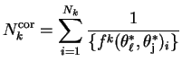
The correction of angular resolution, finite selection efficiency and detector acceptance effects can be made by introducing a correction factor into the calculation of the SDM elements. This correction factor is calculated from the ratio of the number of fully detector simulated, selected Monte Carlo events, to the number of generated Monte Carlo events.
This is done in a bin-wise manner, so a correction factor is calculated for a certain volume of phase space as the ratio of the number of events in that phase space, before simulation and selection, to the number of events after full simulation and selection.
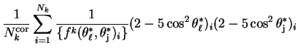
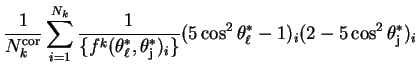
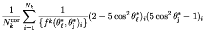
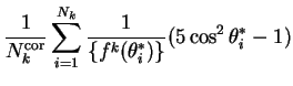
The relevant SDM elements for calculating the W-pair polarised cross-sections
and the individual W polarised
cross-sections are only
functions of the W production angle
![]() , and the polar angle of the W
decay product,
, and the polar angle of the W
decay product,
![]() , so the correction factor only has to be
calculated as a function of these variables.
, so the correction factor only has to be
calculated as a function of these variables.
The correction factor will then be calculated as:
 |
(8.1) |
Where rec denotes the selected, reconstructed cross-section and true denotes
the generated cross-section.
![]() is the folded polar angle
of the decay hadron. The hadronic jet with
is the folded polar angle
of the decay hadron. The hadronic jet with
![]() is
the angle used.
is
the angle used.
![]() is the polar angle of the decay
lepton. If the
is the polar angle of the decay
lepton. If the
![]() distribution is separated into
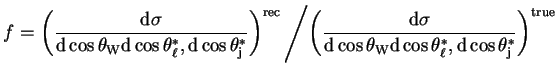
distribution is separated into ![]() bins, then there will be a set of correction factors for each bin of
bins, then there will be a set of correction factors for each bin of
![]() ,
each of which will only be a function of the polar angles of the W decay
products. This correction factor can be applied to the
calculation of the appropriate SDM element as follows:
,
each of which will only be a function of the polar angles of the W decay
products. This correction factor can be applied to the
calculation of the appropriate SDM element as follows:
 |
(8.2) |
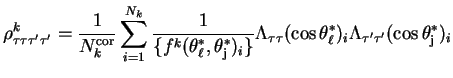
| (8.4) | |||
 |
|||
| (8.5) | |||
 |
|||
| (8.6) | |||
 |
|||
 |
|||
| (8.7) | |||
 |
|||
| (8.8) | |||
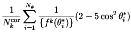 |
The correction factors are calculated from Monte Carlo data. The width of the bins used has to be small enough to give reasonable results, but its width is limited by the resolution of the angular variables. Although the correction is designed to account for events migrating between bins, if the bin width is much less than the resolution, then the correction will be less reliable due to the very large numbers of events migrating between bins. The angular resolutions of the W production and polar decay angles are shown in figure 8.1.
 |
The resolution of
![]() is 0.04, the resolution of
is 0.04, the resolution of
![]() is
0.06 and the resolution of of
is
0.06 and the resolution of of
![]() is 0.08, so the bin
widths have to be larger than these. If the
is 0.08, so the bin
widths have to be larger than these. If the
![]() distribution is once again
divided into 8 equal bins, the width of each will be 0.25, which is much larger
than the resolution. For the polar angles it is important to have more bins as
it is these that are most sensitive to the W polarisation. For the lepton the
bin width is chosen as 0.1, which means that the
distribution is once again
divided into 8 equal bins, the width of each will be 0.25, which is much larger
than the resolution. For the polar angles it is important to have more bins as
it is these that are most sensitive to the W polarisation. For the lepton the
bin width is chosen as 0.1, which means that the
![]() distribution
is split into 20 equal bins in the range [
distribution
is split into 20 equal bins in the range [![]() ,
,![]() ].
For
].
For
![]() a bin width of
0.1 is used in the folded range of [0,
a bin width of
0.1 is used in the folded range of [0,![]() ], thus it is divided into 10
equal bins when calculating the correction factor.
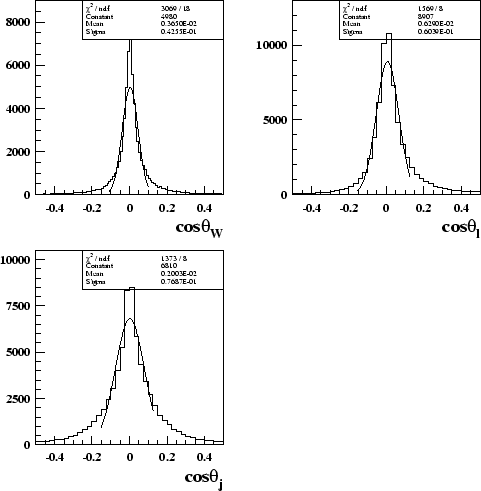
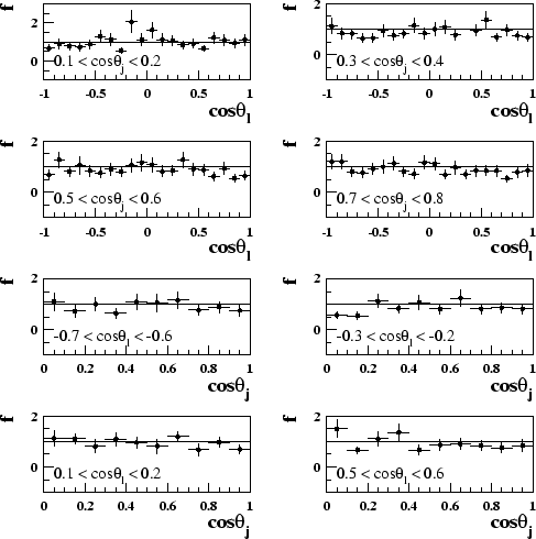
Examples of some of the correction factor distributions are shown in figures 8.2 and 8.3. For the
], thus it is divided into 10
equal bins when calculating the correction factor.
Examples of some of the correction factor distributions are shown in figures 8.2 and 8.3. For the
![]() range [
range [![]() 0.25,0.0] it is
obvious that the correction is limited by Monte Carlo statistics.
0.25,0.0] it is
obvious that the correction is limited by Monte Carlo statistics.
 |
 |
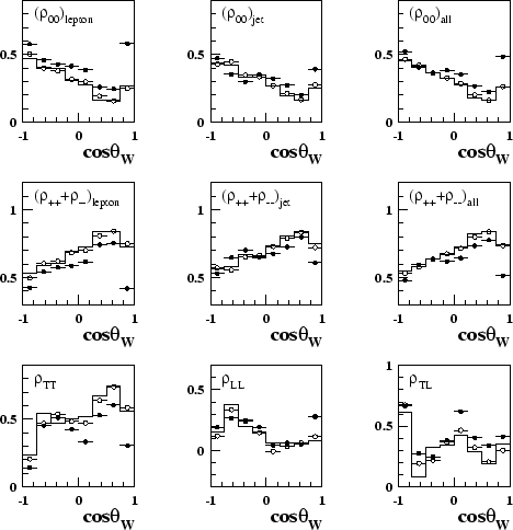
The correction can be tested by applying it to fully simulated Monte Carlo samples. It will obviously correct the EXCALIBUR sample used to calculate the correction factors to extremely good accuracy, but as figure 8.4 demonstrates, it also gives a good approximation of the true SDM elements when applied to a sample of fully simulated PYTHIA Monte Carlo. Figure 8.4 shows the combinations of SDM elements needed to calculate the polarised cross-sections.
 |
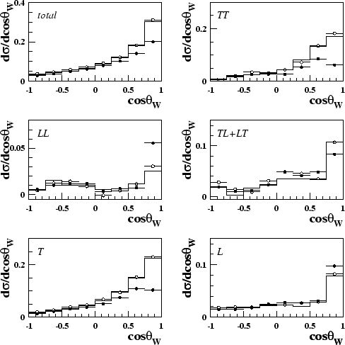
Using these corrected SDM elements to calculate the individual W and W-pair polarised differential cross-sections for the PYTHIA sample, as described by equations 3.38 and 3.33, the plots in figure 8.5 are obtained. Once again, the correction produces a good approximation of the true cross-sections.
 |
Integrating over
![]() on the polarised differential cross-sections gives the
total polarised cross-section. The total polarised cross-section divided by the
total cross-section gives the fraction of each polarisation state. Calculating
these numbers from generator level Monte Carlo and from the corrected
polarised cross-sections will give a quantitative check of the detector
correction. Figure 8.6 shows the calculated fractions from
generator level Monte Carlo and also fully simulated Monte Carlo, both before
and after the detector correction. Shown, are the results for a number of
Standard Model Monte Carlo samples and also some non-Standard Model
samples. It is obvious
that the detector simulation has a large effect on the measured polarised
fraction. In all cases, for both Standard and non-Standard Model Monte Carlo
the detector correction gives results that are within one standard deviation
of the true polarised fractions. It is interesting to note that for all
Monte Carlo samples the detector simulation has a similar effect. The
fraction of TT pairs is decreased and thus the fraction of other polarised
W-pairs is enhanced. This is due to the detector simulation having the largest
effect in the high
on the polarised differential cross-sections gives the
total polarised cross-section. The total polarised cross-section divided by the
total cross-section gives the fraction of each polarisation state. Calculating
these numbers from generator level Monte Carlo and from the corrected
polarised cross-sections will give a quantitative check of the detector
correction. Figure 8.6 shows the calculated fractions from
generator level Monte Carlo and also fully simulated Monte Carlo, both before
and after the detector correction. Shown, are the results for a number of
Standard Model Monte Carlo samples and also some non-Standard Model
samples. It is obvious
that the detector simulation has a large effect on the measured polarised
fraction. In all cases, for both Standard and non-Standard Model Monte Carlo
the detector correction gives results that are within one standard deviation
of the true polarised fractions. It is interesting to note that for all
Monte Carlo samples the detector simulation has a similar effect. The
fraction of TT pairs is decreased and thus the fraction of other polarised
W-pairs is enhanced. This is due to the detector simulation having the largest
effect in the high
![]() region and this is where most of the TT W-pairs
are found, as can be seen for example in figure 8.5.
region and this is where most of the TT W-pairs
are found, as can be seen for example in figure 8.5.
 |
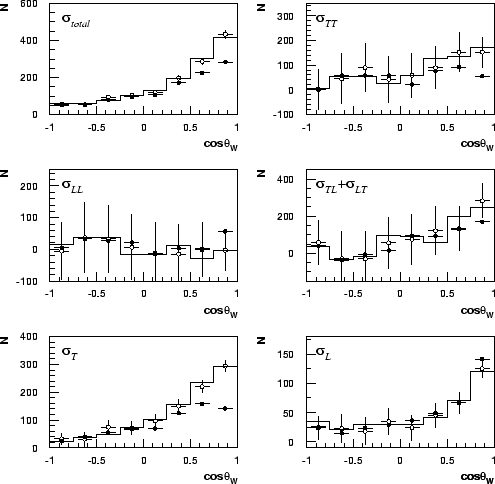
The correction has also been tested on the polarised cross-sections extracted from Monte Carlo subsamples with the same statistics to the data sample. Figure 8.7 shows an example of one of these tests. The correction appears to give a good approximation of the true cross-sections.
 |
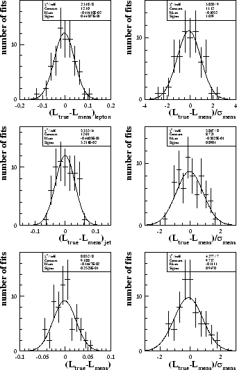
The fractional polarised cross-sections have also been extracted from the subsamples. They were calculated for both the generator level Monte Carlo and the fully simulated Monte Carlo. Figure 8.8 shows the difference between the true (generator level) and measured (fully simulated, corrected) values of the fraction of W bosons with longitudinal polarisation. Results for both the leptonically and hadronically decaying W boson as well as the combined result are shown. Good agreement is seen between the measured and true values. Also shown on figure 8.8 are the pull distributions for these results. The widths are all close to unity, although the width for the hadronically decaying W boson is slightly low, suggesting that the statistical error may be slightly overestimated.
 |
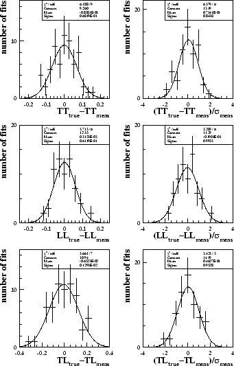
Similar plots for the W-pair polarised cross-sections can be seen in
figure 8.9. Good agreement between the true and measured values is once again seen. The pull distributions all have widths close to unity
except that for
![]() , which is slightly low, again
suggesting a slight
overestimation in the statistical error.
, which is slightly low, again
suggesting a slight
overestimation in the statistical error.
 |
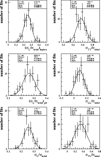
The distributions of the measured values of both the fraction of longitudinal W bosons and the W-pair polarised cross-section fractions can be seen in figure 8.10. The width of these distributions can be taken as the expected statistical error on the measured values.
 |