The Combined Fit

The single W SDM elements and the $\cos\theta_{\rm W}$ distribution are completely uncorrelated. This means that the $\chi ^{2}$s for both fits can be added together. This fit will then include all the observables used in the SDM analysis.

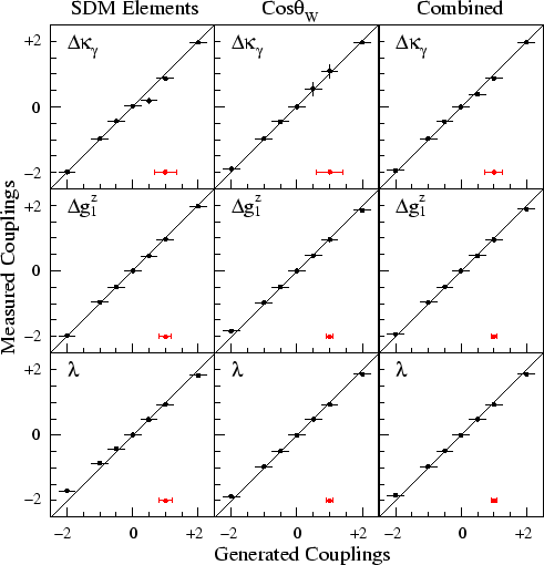
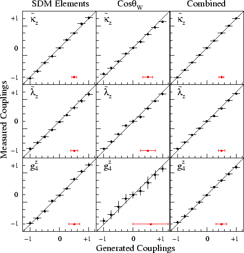
Bias tests performed using this combined fit are shown in table 6.8 and 6.7 and the bias plots are shown in figure 6.4, 6.5 and  6.6. The combined fit gives a noticeable improvement on the fitted values compared to the SDM elements or $\cos\theta_{\rm W}$ distributions on their own.

Table 6.7: The bias fits to large Monte Carlo data samples generated with anomalous CP-conserving couplings using the combined fit. Both reweighting techniques were used. The errors shown are the statistical uncertainty on fit to the large samples.

Coupling	Generated Value	Fitted Value
		WVCXME	BILGOU
$\Delta\kappa_{\gamma}$	$-$2.0	$-$1.95 $^{+0.03}_{-0.03}$	$-$1.94 $^{+0.03}_{-0.02}$
$\Delta\kappa_{\gamma}$	$-$1.0	$-$0.98 $^{+0.03}_{-0.03}$	$-$0.96 $^{+0.03}_{-0.02}$
$\Delta\kappa_{\gamma}$	$-$0.5	$-$0.45 $^{+0.03}_{-0.03}$	$-$0.44 $^{+0.03}_{-0.03}$
$\Delta\kappa_{\gamma}$	0.0	0.0 $^{+0.04}_{-0.03}$	0.0 $^{+0.05}_{-0.04}$
$\Delta\kappa_{\gamma}$	$+$0.5	$+$0.38 $^{+0.06}_{-0.07}$	$+$0.40 $^{+0.06}_{-0.07}$
$\Delta\kappa_{\gamma}$	$+$1.0	$+$0.87 $^{+0.06}_{-0.05}$	$+$0.85 $^{+0.05}_{-0.07}$
$\Delta\kappa_{\gamma}$	$+$2.0	$+$1.99 $^{+0.03}_{-0.03}$	$+$1.97 $^{+0.03}_{-0.03}$
$\Delta g^{z}_{1}$	$-$2.0	$-$1.93 $^{+0.03}_{-0.02}$	$-$1.89 $^{+0.03}_{-0.03}$
$\Delta g^{z}_{1}$	$-$1.0	$-$0.96 $^{+0.02}_{-0.02}$	$-$0.95 $^{+0.02}_{-0.02}$
$\Delta g^{z}_{1}$	$-$0.5	$-$0.49 $^{+0.01}_{-0.01}$	$-$0.49 $^{+0.01}_{-0.01}$
$\Delta g^{z}_{1}$	0.0	0.0 $^{+0.01}_{-0.01}$	0.0 $^{+0.01}_{-0.01}$
$\Delta g^{z}_{1}$	$+$0.5	$+$0.46 $^{+0.04}_{-0.04}$	$+$0.42 $^{+0.03}_{-0.03}$
$\Delta g^{z}_{1}$	$+$1.0	$+$0.95 $^{+0.03}_{-0.03}$	$+$0.95 $^{+0.03}_{-0.03}$
$\Delta g^{z}_{1}$	$+$2.0	$+$1.89 $^{+0.03}_{-0.03}$	$+$1.89 $^{+0.03}_{-0.03}$
$\lambda$	$-$2.0	$-$1.94 $^{+0.03}_{-0.03}$	$-$1.89 $^{+0.02}_{-0.02}$
$\lambda$	$-$1.0	$-$0.97 $^{+0.02}_{-0.02}$	$-$0.97 $^{+0.02}_{-0.02}$
$\lambda$	$-$0.5	$-$0.49 $^{+0.02}_{-0.02}$	$-$0.49 $^{+0.02}_{-0.02}$
$\lambda$	0.0	0.0 $^{+0.01}_{-0.01}$	+0.00 $^{+0.02}_{-0.02}$
$\lambda$	$+$0.5	$+$0.48 $^{+0.03}_{-0.03}$	$+$0.46 $^{+0.02}_{-0.02}$
$\lambda$	$+$1.0	$+$0.93 $^{+0.01}_{-0.01}$	$+$1.03 $^{+0.02}_{-0.02}$
$\lambda$	$+$2.0	$+$1.96 $^{+0.02}_{-0.02}$	$+$1.98 $^{+0.02}_{-0.02}$

Table 6.8: The bias fits to large Monte Carlo data samples generated with anomalous CP-violating couplings using the combined fit. The errors shown are the statistical uncertainty on fit to the large samples.

Coupling	Generated Value	Fitted Value
		WVCXME	BILGOU
$\tilde{\kappa}_{z}$	$-$1.00	-	$-$1.01 $^{+0.02}_{-0.02}$
$\tilde{\kappa}_{z}$	$-$0.50	-	$-$0.50 $^{+0.02}_{-0.02}$
$\tilde{\kappa}_{z}$	$-$0.25	-	$-$0.25 $^{+0.01}_{-0.01}$
$\tilde{\kappa}_{z}$	0.0	-	$-$0.01 $^{+0.01}_{-0.01}$
$\tilde{\kappa}_{z}$	$+$0.25	-	$+$0.24 $^{+0.01}_{-0.01}$
$\tilde{\kappa}_{z}$	$+$0.50	-	$+$0.50 $^{+0.02}_{-0.02}$
$\tilde{\kappa}_{z}$	$+$1.00	-	$+$1.00 $^{+0.02}_{-0.02}$
$\tilde{\lambda}_{z}$	$-$1.00	-	$-$0.93 $^{+0.03}_{-0.03}$
$\tilde{\lambda}_{z}$	$-$0.50	-	$-$0.46 $^{+0.02}_{-0.02}$
$\tilde{\lambda}_{z}$	$-$0.25	-	$-$0.24 $^{+0.02}_{-0.02}$
$\tilde{\lambda}_{z}$	0.0	-	0.0 $^{+0.02}_{-0.02}$
$\tilde{\lambda}_{z}$	$+$0.25	-	$+$0.18 $^{+0.02}_{-0.02}$
$\tilde{\lambda}_{z}$	$+$0.50	-	$+$0.44 $^{+0.03}_{-0.03}$
$\tilde{\lambda}_{z}$	$+$1.00	-	$+$0.94 $^{+0.03}_{-0.03}$
$g^{z}_{4}$	$-$1.00	-	-0.94 $^{+0.05}_{-0.05}$
$g^{z}_{4}$	$-$0.50	-	$-$0.48 $^{+0.04}_{-0.04}$
$g^{z}_{4}$	$-$0.25	-	$-$0.25 $^{+0.04}_{-0.05}$
$g^{z}_{4}$	0.0	-	$-$0.01 $^{+0.04}_{-0.04}$
$g^{z}_{4}$	$+$0.25	-	$+$0.26 $^{+0.04}_{-0.04}$
$g^{z}_{4}$	$+$0.50	-	$+$0.49 $^{+0.04}_{-0.04}$
$g^{z}_{4}$	$+$1.00	-	$+$0.94 $^{+0.04}_{-0.04}$

Figure 6.4: Bias plots of the CP-conserving TGC fits using the WVCXME reweighting scheme. The first column is the fit to the SDM elements, the second column is the fit to the W production angle, and the third column is the combined fit. The solid line represents the perfect fit. The red points represent the expected statistical error on the data.

Figure 6.5: Bias plots of the CP-conserving TGC fits using the BILGOU reweighting scheme. The first column is the fit to the SDM elements, the second column is the fit to the W production angle, and the third column is the combined fit. The solid line represents the perfect fit. The red points represent the expected statistical error on the data.

Figure 6.6: Bias plots of the CP-violating TGC fits using the BILGOU reweighting scheme. The first column is the fit to the SDM elements, the second column is the fit to the W production angle, and the third column is the combined fit. The solid line represents the perfect fit. The red points represent the expected statistical error on the data.