Fit to Many Subsamples

Fitting to subsamples of Monte Carlo with the same statistics as the data sample will give a test of the reliability of the statistical error calculated for the fit. For the error to be reliable 67% of the fitted coupling values should lie within one standard deviation of the generated value. If this is true, then the distribution of $\frac{x-x_{0}}{\Delta x}$ , where

is the fitted value of the coupling, $x_{0}$ is the generated value and $\Delta x$ is the statistical error on

, should be a Gaussian with a width consistent with unity. These distributions are known as the pull distributions.

These tests were performed for all six couplings being measured, using both reweighting methods where applicable. Fits were not only made to Standard Model Monte Carlo but also samples with all the anomalous couplings used in the bias tests. A summary of the results is shown below.

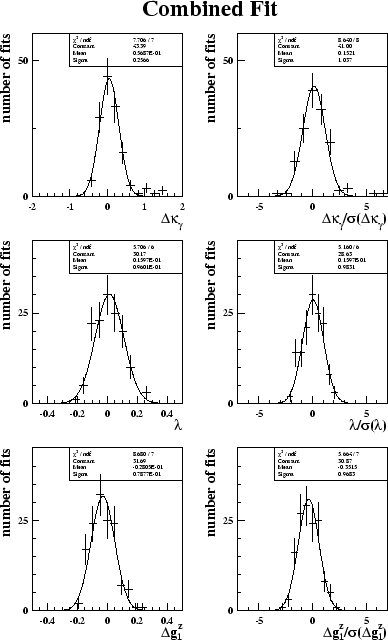
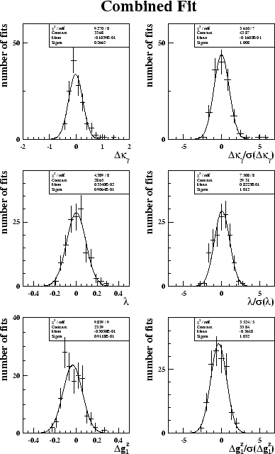
Figure 6.7 shows the distributions of fitted values of the CP-conserving couplings. The fits were made to 139 Standard Model subsamples using the BILGOU reweighting scheme, and are for the combined fit result. The plots on the left just show the distributions and demonstrate that the fit is Gaussian and the mean is at the Standard Model value of the couplings. The width of this distribution can be taken as the expected statistical error on the measured value of the coupling. The plots on the right are the pull distributions. Figure 6.8 shows the distributions of the combined fit of the CP-conserving couplings, using the WVCXME reweighting scheme. For both reweighting methods the width of the pull distributions is close to unity for all couplings.

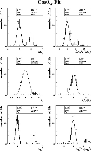
For both reweighting schemes, the fits for $\Delta\kappa_{\gamma}$ show a number of results with a large deviation from the generated value of coupling. These generally take a value greater than $\Delta\kappa_{\gamma}$ =

1. This is because the $\cos\theta_{\rm W}$ distribution for $\Delta\kappa_{\gamma}$ =

2 is the same as that for the Standard Model. The plots of fits to just the $\cos\theta_{\rm W}$ distribution for the CP-conserving couplings, using the BILGOU reweighting scheme are shown in figure 6.9. For the fits to $\Delta\kappa_{\gamma}$ it is obvious that a large proportion of the samples are mistakenly fitted as $\Delta\kappa_{\gamma}$ =

2. A similar effect is seen to a lesser extent in the $\Delta g^{z}_{1}$ fits to $\cos\theta_{\rm W}$ , where the $\cos\theta_{\rm W}$ distribution at about $\Delta g^{z}_{1}$ =

1 is similar to that of the Standard Model.

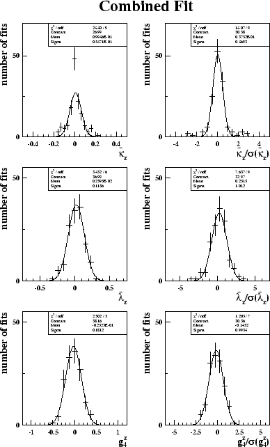
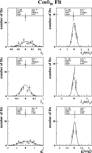
Figure 6.10 shows the distributions of the fitted values of the CP-violating couplings for the combined fit using the BILGOU reweighting scheme. The distribution for $\tilde{\kappa}_{z}$ does not appear Gaussian, and there is a bias towards a coupling of zero. This is because any anomalous CP-violating coupling will cause a flattening in the $\cos\theta_{\rm W}$ distribution. Due purely to statistical fluctuations, a number of the subsamples will have $\cos\theta_{\rm W}$ distributions that are steeper than the Standard Model distribution. The fits of the CP-violating couplings to these subsamples will immediately be biased towards zero and the fits using just the $\cos\theta_{\rm W}$ distribution will all give a coupling value of zero. This obvious bias only manifests in the $\tilde{\kappa}_{z}$ fit and not those of the other two CP-violating couplings. This is because the W production angle is much less sensitive to $\tilde{\lambda}_{z}$ and $g^{z}_{4}$ than $\tilde{\kappa}_{z}$ , so for these the SDM element fits completely dominate in the combined fit results.

Figure 6.11 shows the distributions of the fit of the CP-violating couplings to just the $\cos\theta_{\rm W}$ distribution. It can be seen that in all coupling fits there is a large spike at zero demonstrating the effect discussed.

The pull distributions for the combined fit of $\tilde{\kappa}_{z}$ , shown in figure 6.10, has a width much less than unity, as would be expected. This then means that the width of the distribution of fitted values cannot be taken as the expected error. For all the CP-violating couplings the expected error has been taken as the mean value of the statistical error from all the fits to the subsamples.

Table 6.9 shows the expected value of the statistical error that should be calculated in the fits to the OPAL data.

**Figure 6.7:** Combined fit results to 139 subsamples of Standard Model EXCALIBUR Monte Carlo. The BILGOU reweighting scheme was used in the fits. The widths of the distributions of the plots on the left side represent the expected error for the analysis for the corresponding coupling parameters. The width of the pull distributions, the plots on the right side, should be compatible with unity if the statistical error is reliable.
$\begin{figure}\begin{center} \epsfig{file=figs/pull_sm_combined.eps,width=0.8\linewidth}\end{center}\end{figure}$

**Figure 6.8:** Combined fit results to 139 subsamples of Standard Model EXCALIBUR Monte Carlo. The WVCXME reweighting scheme was used in the fits. The widths of the distributions of the plots on the left side represent the expected error for the analysis for the corresponding coupling parameters. The width of the pull distributions, the plots on the right side, should be compatible with unity if the statistical error is reliable.
$\begin{figure}\begin{center} \epsfig{file=figs/pull_sm_wvc.eps,width=0.8\linewidth}\end{center}\end{figure}$

**Figure:** $\cos\theta_{\rm W}$ fit results of 139 subsamples to Standard Model EXCALIBUR Monte Carlo. The BILGOU reweighting scheme was used for these fits The widths of the distributions of the plots on the left side represent the expected error for the analysis for the corresponding coupling parameters. The width of the pull distributions, the plots on the right side, should be compatible with unity if the statistical error is reliable.
$\begin{figure}\begin{center} \epsfig{file=figs/pull_sm_cos.eps,width=0.8\linewidth}\end{center}\end{figure}$

**Figure 6.10:** Combined fit results for the CP-violating couplings to 139 subsamples of Standard Model EXCALIBUR Monte Carlo. The plots on the left are the distributions of fitted values and the plots on the right are the pull distributions.
$\begin{figure}\begin{center} \epsfig{file=figs/pull_sm_cp.eps,width=0.8\linewidth}\end{center}\end{figure}$

**Figure:** $\cos\theta_{\rm W}$ fit results for the CP-violating couplings to 139 subsamples of Standard Model EXCALIBUR Monte Carlo. The plots on the left are the distributions of fitted values and the plots on the right are the pull distributions.
$\begin{figure}\begin{center} \epsfig{file=figs/pull_sm_cos_cp.eps,width=0.8\linewidth}\end{center}\end{figure}$

Table 6.9: The expected statistical error of the fit to the TGC parameters. These were calculated from the fits to many Monte Carlo subsamples. For the CP-conserving TGCs, the first three are using the BILGOU reweighting scheme and the next three are using the WVCXME scheme.

Coupling	SDM elements	$\cos\theta_{\rm W}$ distribution	Combined
$\Delta\kappa_{\gamma}$ $^{(BG)}$	0.321	0.335	0.257
$\lambda$ $^{(BG)}$	0.184	0.100	0.096
$\Delta g^{z}_{1}$ $^{(BG)}$	0.205	0.111	0.079
$\Delta\kappa_{\gamma}$ $^{(WVC)}$	0.336	0.401	0.266
$\lambda$ $^{(WVC)}$	0.192	0.106	0.091
$\Delta g^{z}_{1}$ $^{(WVC)}$	0.186	0.096	0.091
$\tilde{\kappa}_{z}$	0.090	0.174	0.084
$\tilde{\lambda}_{z}$	0.122	0.259	0.110
$g^{z}_{4}$	0.184	0.700	0.180