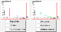
Job Traversal Times
Last Completion Times
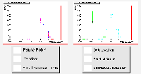
Number of Transfers
The work carried out so far with EDGSim has had two main purposes: comparing the performance of different scheduling algorithms, and checking that the performance of the simulation is convincing. Constructing a realistic "testbed" and distribution of jobs is not easy, since there is no fully operational European Data Grid as yet for comparison. These experiments were carried out with best-guess figures for many of the parameters of such a grid.
The six resource matching algorithms tested in this work selected CEs based on the following:
The grid for the first experiments was chosen to be a homogenous one, with ten identical nodes (other than one that additionally hosted the Resource Broker and the Replica Catalog). These each contained a Compute Element managing ten identical worker machines, and a Storage Element with 50 1GB files stored and 200GB cache space for temporary files. The maximum bandwidth between any two sites was 0.01GB / sec.
The jobs themselves were chosen to be identical, except for the required input data, consisting of ten randomly selected files. The jobs required 5000 seconds (on the CPUs available in this virtual grid) to run over each data file. Memory dependency was factored out by giving the jobs memory requirements that were less than the memory available on the worker machines. Only one job was run at a time on any machine. The jobs were generated at Poisson distributed intervals with an average of 300 seconds. Job generation stopped at 10000 seconds from the start time, and the simulation then ran until all jobs were completed. The simulation was run 100 times for each scheduler.
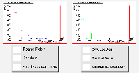
The plots below are:
The results of the six schedulers are separated onto two plots in each set for the sake of clarity.
|
Job Traversal Times |
Last Completion Times |
Number of Transfers |
Surprisingly, the round-robin scheduler gives the best performance here, looking at the job processing times in the first two plots. It was included for the sake of comparison as the simplest load-sharing algorithm, passing jobs one at a time to the resources available. It could be expected that any algorithm making any intelligent decision, particularly one that responds to feedback from the system, would perform better.
The reason for this is the slightly artificial nature of this experiment. The more symmetrical the grid setup, the better the performance given by the round-robin algorithm. This Grid is about as symmetrical as possible, consisting of ten identical nodes with ten identical machines each. The effect is enhanced by the identically-sized jobs.
The estimated traversal time algorithm is the only one that can compete. This may be partially due to the fact that it relies on the round-robin algorithm until feedback begins to arrive from the first jobs to be completed. The others do little or no better than the random algorithm, as there is little to choose between the identical sites, which will be returning very similar results, and all of these dynamic algorithms are forced to make a random choice if there is a tie between two or more sites. The round-robin algorithm is in fact the only one that does not make random choices at any point.
The two algorithms that attempt to send jobs to the location of the most required data show their worth in a plot of the number of transfers made per run. Here it can be seen that they lead to a roughly 15% reduction in transfers made. The time taken for a file to transfer is negligible compared to the time taken for the job to run in this experiment, which is why these algorithms still perform poorly in terms of job processing times.
Another effect caused by the symmetry of this grid can be seen in the peaked structure of the job traversal times. These peaks occur approximately every 50 000 seconds, corresponding the the time needed to run a job. The peak that a given job falls into depends on how many jobs were ahead of it in the queue. Job processing, and the emptying of the queue, happen at the same rate at each of the (identical) sites, producing the peaks.
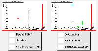
In order to break this symmetry and remove these slightly unrealistic effects, the jobs were given a Gaussian distribution in CPU time requirements. This distribution had a mean of 50 000 seconds, and also a standard deviation of 50 000 seconds, truncated to a minimum size of 500 seconds, and a maximum of 100 000 seconds. The results are shown below:
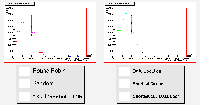
Job Traversal Times |
Last Completion Times |
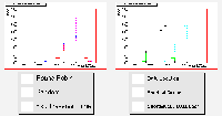
Number of Transfers |
It can immediately be seen that the performance of the estimated traversal time algorithm has collapsed. In the last completion time results particularly, this algorithm has fallen a long way behind even the random algorithm, which even the simplest load balancing techniques should be able to beat.
This is happening because of the algorithm's dependency on previous job results. The estimate is based on previous traversal times, with some scaling involving queue lengths. However the jobs are now varying in the amount of time needed to run, which means that these previous values are no longer a reliable guide, as a job's traversal time is dominated by processing time.
If a CE is given a very small (in CPU seconds) job to process, it will inevitably return a very favourable traversal time to the RB via the Information Services. This will lead to a misleadingly small estimate of future traversal times, and the scheduler will send any incoming jobs to this resource. In fact, until this resource returns any more results, all jobs are likely to be sent here regardless of whether it is already overloaded. This is likely to mean that the decisions made by the RB are actually counterproductive, and lead to a worse performance than even a random scheduler.
The round-robin scheduler is still competing well, despite the varying job sizes, as the resources are still identical, and the differences appear to be evened out over a given run. However the algorithms which choose the CE with the shortest queue are now performing just as well, balancing any unequal load on the grid.
The data location scheduler continues to give poor job processing results, but a significant reduction in network load. Much more successful is the algorithm that combines this with selection of resources based on queue length. This produces job processing results that compare favourably with any of the others, but also reduce the network load. The combination of these two simple algorithms makes efficient use of the computing resources, and still processes jobs at a favourable rate.
It is also worth noting that as expected, the variation in job sizes has removed the peaked structure in the job traversal times.