Non-destructive measurements of beam position are essential for the effective running of any modern accelerator. A number of different types of device exist for just such a purpose that come under the generic title Beam Position Monitor, or BPM. Each of these types of BPM makes use of the coupling of the electromagnetic field around a charged particle bunch to some sort of conductor, although the methods used for extracting this signal from the BPM vary and are largely dependent upon the type of BPM used. Three of the most common types of BPM used in modern accelerators are:
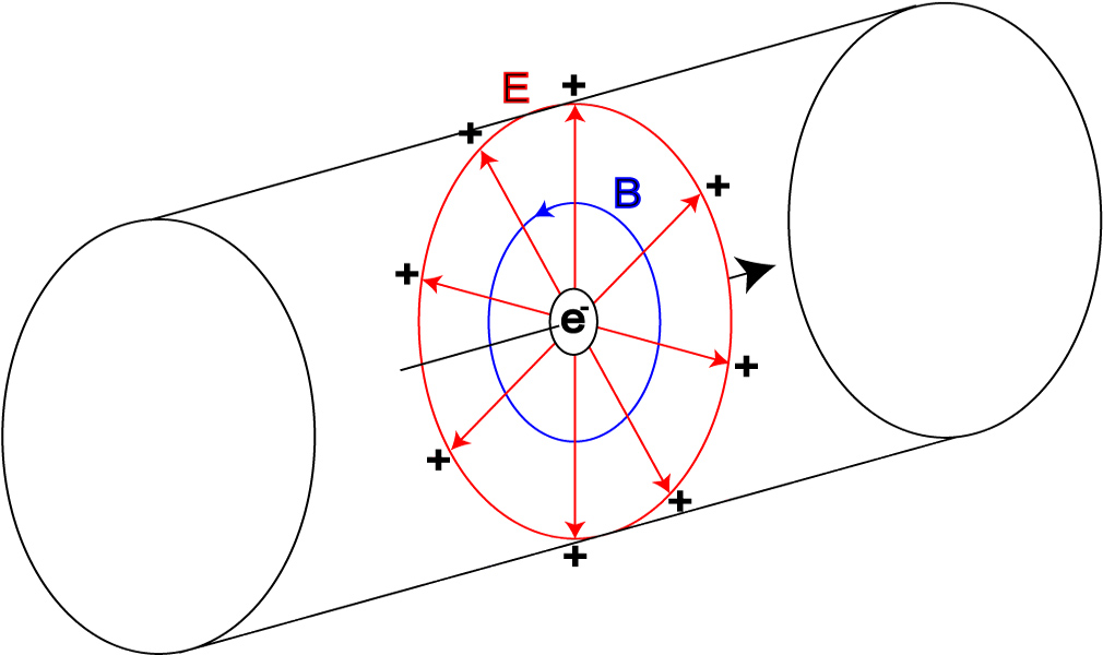
| Figure 4.1: Field lines and image charge due to a charged particle beam. |
The stripline BPM is essentially a variation on the button, in which the EM-field lines surrounding a charged bunch terminate on some sort of pickup. In contrast, a cavity BPM uses an appropriately shaped RF cavity that is resonant at the bunching frequency. A resonant EM-field is then set up within the cavity as a result of the passing bunch. In each case, the BPM makes use of the EM-field that surrounds the charged particle bunch and its corresponding image charge: this is shown in Fig. 4.1. The image charge that appears on the beam pipe wall results from the termination of the E-field on the conducting beam pipe. In the relativistic limit (v → c), Lorentz contraction of the EM-field means that there is essentially no longitudinal component to the field, resulting in purely transverse electric and magnetic fields [61].
For a beam centred in the beam pipe, this image charge is evenly distributed over the whole circumference of the pipe and travels along the pipe with the charge, as shown in Fig. 4.1. For an electrode mounted on the beampipe wall, with an angular coverage φ, the induced current in the electrode is therefore:
| (4.1) |
for a beam current Ibeam. It is the termination of the field on the electrodes, in place of the beampipe wall, that gives rise to an induced signal on the electrode. For an off-centre beam, the density of field lines, and hence the image charge distribution, changes accordingly. For beams located close to the centre of the beampipe, small changes in beam position (on the scale of the beampipe width) produce a change in image charge at the electrode that is approximately linear [78]. Each type of BPM makes use of this change in image charge distribution in a different way.
The Button BPM is the simplest of the three types of beam position monitor. It consists of a pair of electrodes, for each axis in which the beam position is to be measured, on opposing sides of the beampipe. Although a simple antenna would suffice, the electrode for a button BPM is usually small and circular, hence the name [61]. The current from the button as a result of the image charge is a function of both the button area A and the charge density of the image charge ρ:
| (4.2) |
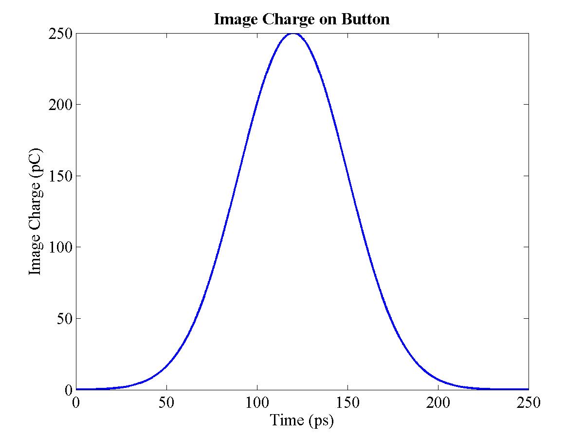
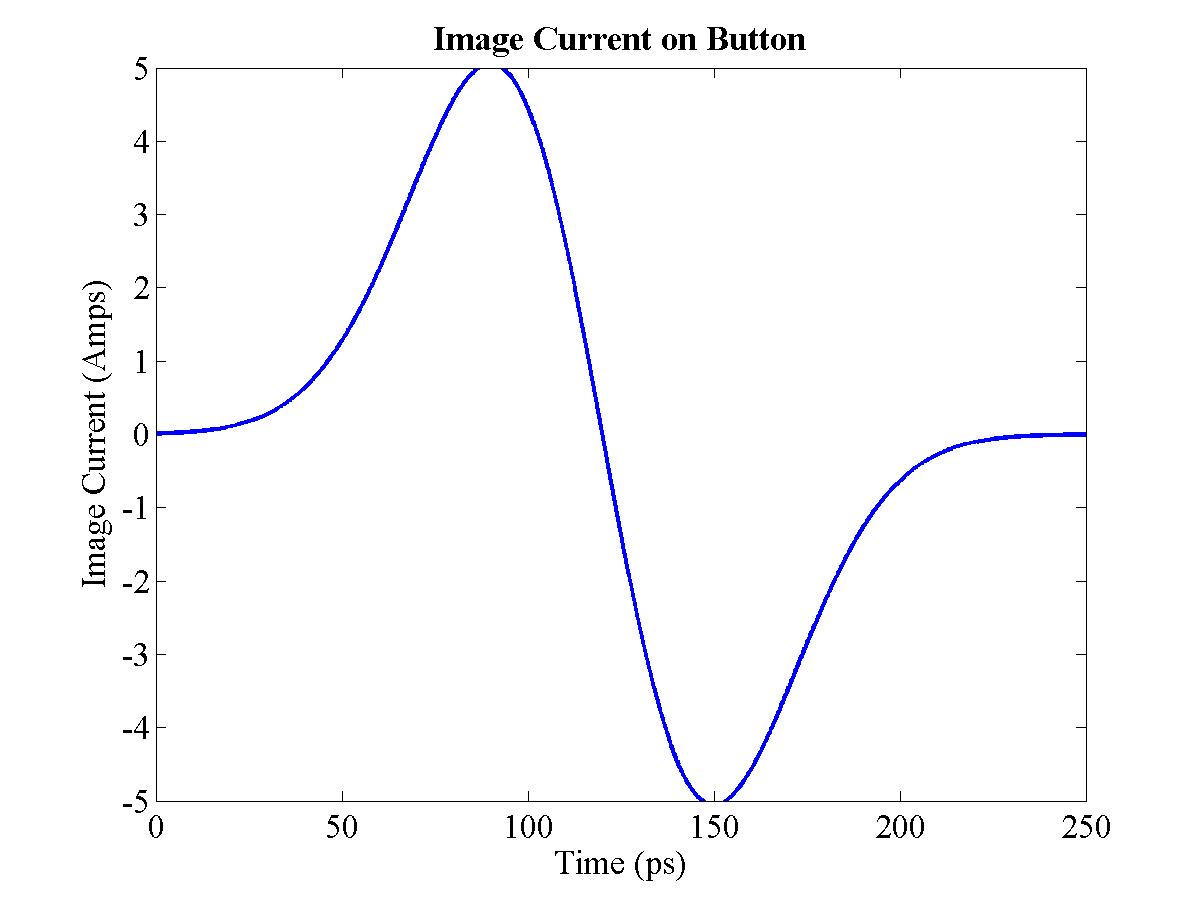
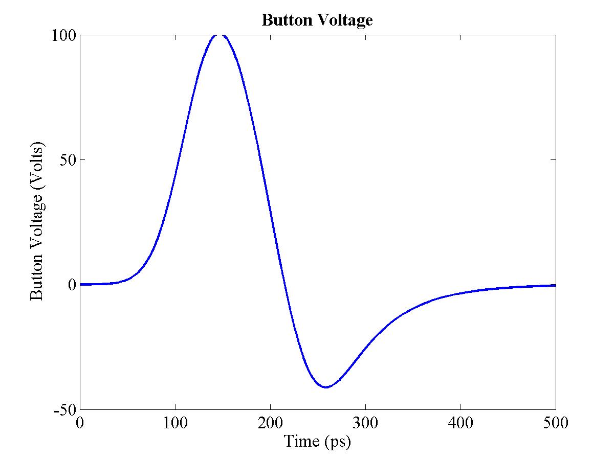
where C is the circumference of the beampipe [79]. The image charge and current on a button are shown in Figs. 4.2(a) and (b) respectively; note that the image current is just the derivative if the image charge. The resulting voltage out of the button is therefore the image current on the button driven into the impedance of the transmission line used to extract the signal from the BPM, plus the impedance from the BPM itself; this impedance also includes the natural capacitance of the BPM, giving a filter-like profile for the voltage response [80]. This is shown in Fig. 4.2(c).
|
|
||||
| (a) Image charge on button | (b) Image current on button | ||||
 |
|||||
| |||||
|
|||||
Having found the signal from a single pickoff of the BPM, it is necessary to combine the information from each of the pickoffs to extract the beam position. As mentioned in Section 3.3, the signal that is produced by a single pickoff is a convolution of both beam proximity and bunch charge. There are a number of different methods of charge subtraction and position normalisation: the most common are difference-over-sum (Δ/Σ), amplitude-to-phase conversion (AM/PM) and log-ratio processing [61]. Amplitude-to-phase conversion involves converting the two pickoff signals into two signals with identical amplitude, but a relative phase difference that is related to the initial amplitude difference between the two signals [81]. Recombining these two signals of equal amplitude but different phase produces a signal whose amplitude is proportional to the amplitude difference of the raw pickoff signals. Log-ratio processing uses a single hybrid to output a signal that is proportional to the logarithm of the ratio of the two input signals [82].
However, the most popular method of BPM signal processing is difference-over-sum. As given in Eq. (3.4), the difference of the two pickoff signals is divided by the sum of the two signals, giving an output that is a) independent of bunch charge and b) approximately proportional (close to the beampipe centre) to the position variation from the centre of the beampipe:
| (4.3) |
for two pickoffs T and B. The usual procedure is to filter each of the signals at the bunching frequency (or, if cost is an issue, at some lower frequency30) and follow the same processing procedure as outlined in Section 3.3, before calculating Δ/Σ to give the actual beam position.
The stripline BPM is a modification of and improvement over the button BPM. Although it is restricted to bunched beams of a particular bunching frequency, it has a significantly better response at that frequency than the button BPM. A standard stripline BPM replaces the button electrodes of a button BPM with long strips that run parallel to the beam direction; an example is shown in Fig. 4.3. The front (upstream) end of the strip is connected, via an appropriate feedthrough, to a transmission line and thence to the BPM processor. The downstream end is either terminated (usually with a 50 Ω terminator) or left as open circuit. The description below is given for the open circuit version; the treatment for a terminated strip is slightly different, but the resulting signal is the same [56].
|
Figure 4.3: Schematic diagram of a stripline BPM used in the SLC. The BPM consists of four strips — |
For a bunched beam of electrons, the signal from a stripline is as follows. As the bunch passes the front end of the stripline, the image charge passes from the beampipe wall onto the strip. The arrival of the image charge causes a charge separation in the strip: positive charge collects on the inner surface of the strip, forming the image charge, and tracks the actual bunch down the strip as the bunch passes through the BPM. The remaining negative charge that is left from this charge separation is free to move and runs in two directions: half follows the image charge down the strip, while the other half passes out through the transmission line. As such, a negative spike is measured as the electron bunch passes the front of the strip.
Once the bunch passes the end of the strip, the image charge reappears on the wall of the beampipe and continues on as usual. At this point, the positive charge on the inner surface of the strip reflects off the rear end of the strip and travels back towards the front end of the strip, accompanied by the remaining half of the negative charge. Once this charge reaches the front of the strip again, a positive spike of equal magnitude to the initial negative spike is registered. If the length of the stripline is exactly 1/4 of the bunch spacing, the reflected signal arrives exactly half a cycle after the initial beam signal. For a CW bunched beam, this produces the response as shown in Fig. 3.6 [56].
The stripline is therefore resonant at the bunching frequency and produces a very strong signal when filtered at this frequency. For strips of length L, the response of the stripline BPM has the following frequency dependence:
| (4.4) |
As such, the frequency response of the BPM contains peaks at the fundamental bunching frequency and odd harmonics thereof [56]. At even harmonics there are troughs in the frequency spectrum: these are caused by the reflected spikes arriving back at the front of the strip at exactly the same time as a new bunch arrives, cancelling the signal. One therefore designs the dimensions of the stripline around the bunch spacing. This makes it difficult to use a stripline BPM for bunching frequencies much above 1 GHz, particularly from the point of view of impedance matching (necessary to ensure there are no reflections between the strip and transmission line). The methods of BPM signal processing for producing a usable position signal are the same as for the button BPM.
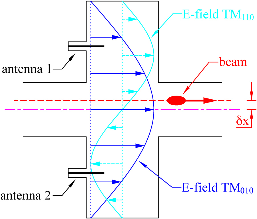
The operation of a cavity BPM is markedly different from the two types of BPM previously described. A cavity BPM takes advantage not of the direct coupling of the EM-field surrounding a bunch to an electrode, but of the ability of a moving bunch to induce an EM-field within a resonant cavity. The cavity is designed to resonate at the bunching frequency of the beam: each bunch that passes through the cavity adds to the resonant field. The behaviour of the EM-field within a resonant cavity is the same as that for a waveguide (see Section 2.3.3). As such, there are a large number of modes at which the EM-field within the cavity can resonate; the magnitudes of each of these modes of oscillation depend on a number of factors, including beam trajectory and the dimensions of the cavity [85]. The two most important modes for the measurement of beam position are the TM010 (monopole) mode and the TM110 (dipole) mode. A cross-section of a cavity BPM, showing the electric fields for the TM010 and TM110 modes is shown in Fig. 4.4.
| Figure 4.4: The TM010 (Monopole) and TM110 (Dipole) modes for a resonant cavity BPM in response to a passing bunch [78]. The dipole mode is only excited for non-zero δx. |
The fundamental mode driven by the bunched beam within the cavity is the monopole mode. However, from the point of view of a beam position measurement, the mode of choice is the dipole mode. The amplitude of the dipole mode depends linearly on the radial beam offset from the cavity centre, and is zero for a beam centred within the cavity [85]. By contrast, the monopole mode is excited most strongly for a centred beam and has no such linear amplitude dependence. Therefore one usually designs the cavity in such a way as to be able to couple out the dipole mode whilst ignoring or damping out the monopole mode: this is done either with the placement of the output coupler (used to extract the beam position signal from the cavity), by coupling out the monopole mode with a coupler that is insensitive to the dipole mode or by using a filter with a narrow bandwidth on the output to select only the frequency of the dipole mode. The position signal can then be measured by using an antenna within the cavity that couples preferentially to the dipole mode (see Fig. 4.4).
The noticeable advantage of a cavity BPM over striplines or buttons is its inherently better position resolution [85]: this is due to the dipole mode signal produced by the cavity. With effective damping and coupling out of the monopole mode, the cavity BPM produces a dominant signal (from the dipole mode) that is only present for an off-centre beam. In contrast, striplines and buttons have to extract this dipole signal from the enormous monopole signal: the electrodes for these BPM types register a signal whether the beam is off-centre or not, meaning that a very small signal (corresponding to an off-centre beam) must be extracted from two very large ones (the raw electrode signals) [86]. This can give an order of magnitude improvement in position resolution for cavities over striplines [87].
It is also possible to improve the position sensitivity of the cavity by increasing the Q through careful design and machining [85]. The Q of a cavity (or a filter) is defined as the ratio of the central frequency to the bandwidth; therefore a 10 GHz cavity with a 10 MHz bandwidth will have Q = 1000. However, the corresponding disadvantage of high-Q cavities is the comparatively poor timing resolution: the large Q causes a corresponding increase in the rise time of the signal. For a bunch train, it is therefore only possible to deconvolve the position of each successive bunch by analysing the signal for the entire train. The output signal from the cavity is effectively the integral over the whole train of the position of each bunch [56]. In addition, a high Q increases the sensitivity of the cavity to external influence, such as physical deformation or external temperature variation. Such external influence can lead to a change in the resonant or coupling frequency of the cavity and hence a change in the measured beam position [85].
As part of the FONT system design, it was necessary to find a BPM best suited to both the NLCTA beam conditions and the FONT requirements. The operating parameters for a FONT BPM are as follows:
All three of the BPM types detailed in Section 4.1 were considered as a possible option for a FONT BPM. The first possibility was to use the existing NLCTA stripline BPM's, or some modification of this design. Within each of the quadrupoles of the NLCTA resides a stripline BPM, of the type shown in Fig. 4.3. The striplines are designed to be resonant at 714 MHz, with a stripline length of 10.5 cm. However, this automatically disqualifies these BPM's from use: a stripline BPM, with electrodes of length L, has peaks in frequency space at odd harmonics of the fundamental frequency (
Also available was the option to use a series of NLC X-band cavity BPM's, developed by Steve Smith and Zenghai Li at SLAC. The intention was to test these cavity BPM's on the NLCTA, giving the possibility of integrating this test with the FONT program by utilising one as the FONT feedback BPM. However the inherent problems with using cavity BPM's ruled them out. Firstly, the rise time associated with a high-Q cavity is such that it would be impossible to resolve beam position on a bunch-by-bunch basis, which is essential for FONT. Secondly, the processing scheme required for a cavity is very different from that for a stripline BPM (and hence the IPFB design), meaning that the use of a cavity BPM would automatically exclude the use of the intended BPM processing scheme.
The best available option was therefore to construct a simple button BPM, designed specifically to be resonant at X-band. It was suggested that it would be possible to tune the pickup antennas of a button BPM to be strongly resonant at X-band and therefore give an enhanced response to the NLCTA beam [30]. It also became clear that constructing a BPM of this kind would be possible from commercially available vacuum components. A design was conceived by Marty Breidenbach and Josef Frisch at SLAC; that design is detailed in the following section.
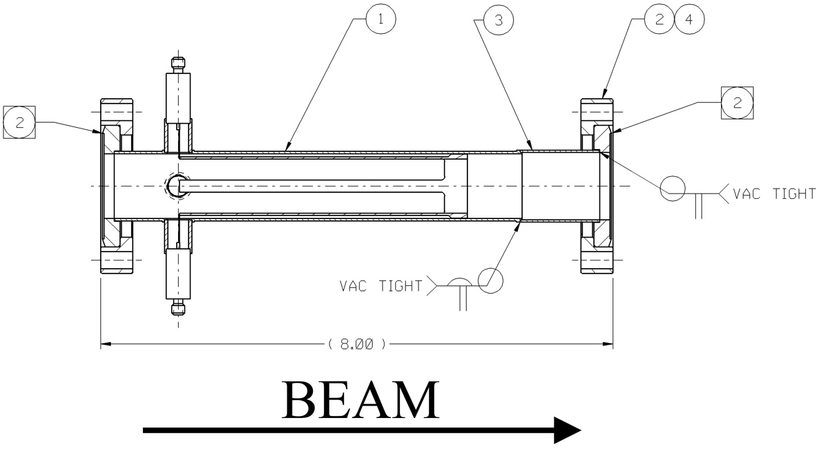
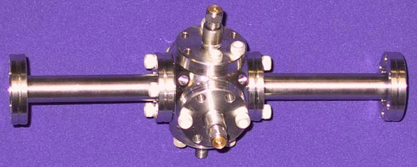
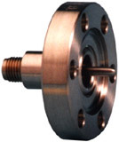
| Figure 4.5: The X-band BPM designed for use in FONT at the NLCTA. The central spherical cube has 6 ports: four are used for position electrodes, with the other two used for the beampipe flanges. |
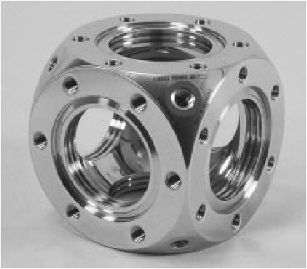
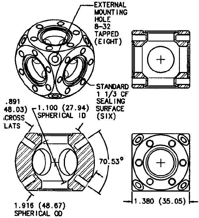
The FONT X-band BPM is shown in Fig. 4.5. The BPM consists of a number of standard vacuum components, all of which are commercially available. The main BPM cavity, to which all the other components are attached, is called a spherical cube; details are shown in Fig. 4.6. The spherical cube used for the X-band BPM is approximately 1.38 in. (35 mm) in diameter and was purchased from Kimball Physics31. On each of its six external faces it has a 1-1/3 in. (34 mm) ConFlat flange vacuum mount, used to attach other vacuum components. Mounted on four of the six faces are four SMA feedthroughs, which act as the electrodes for the BPM; these are shown in Fig. 4.7 and were purchased from Kurt J. Lesker Co. These are mounted using the same 1-1/3 in. ConFlat flanges, each with a vacuum-sealing copper gasket. One opposing pair of these electrodes is used to measure the x signal, with the second pair used for y. The final pair of faces on the spherical cube were used to mount the spool pieces that connect the BPM to the main beampipe, again using copper gaskets to seal the join.
|
|
||||
| (a) Spherical Cube | (b) Spherical cube dimensions | ||||
|
|||||
|
|
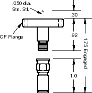
||||
| (a) SMA feedthrough | (b) SMA feedthrough dimensions | ||||
| |||||
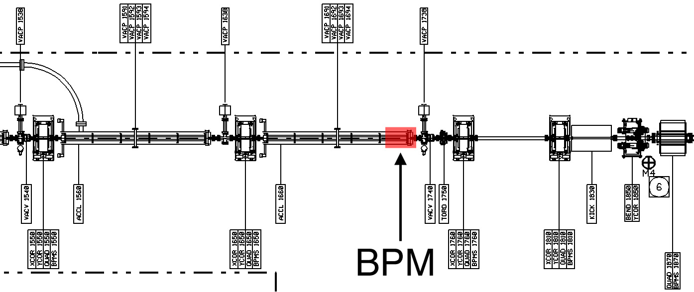
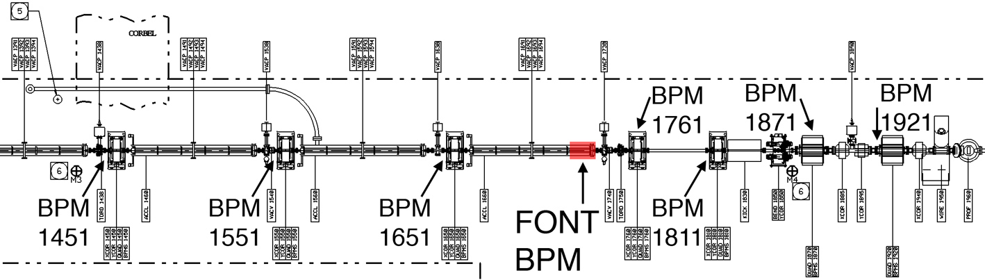
| Figure 4.8: A blow-up of the NLCTA ground plan (Fig. 3.25) showing the location of the FONT BPM. |
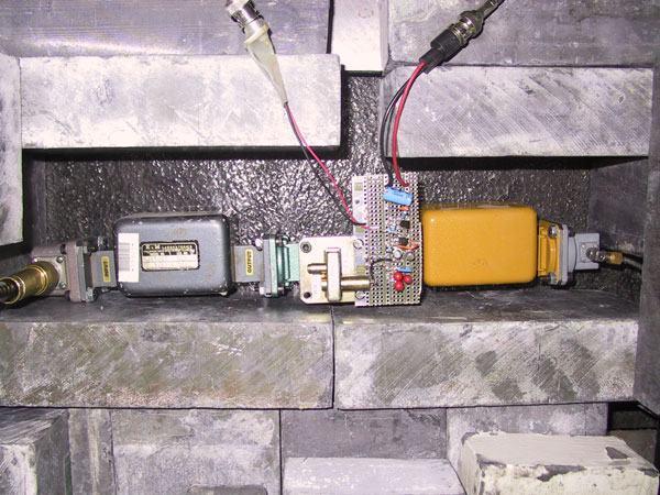
The BPM was installed on the NLCTA downstream of the test structures, upstream of quadrupole QD1760 on girder 17. Fig. 4.8 shows the location of the BPM on the NLCTA. The position of the BPM was advantageous for the FONT experiment as it was located just upstream of one of the NLCTA striplines, mounted inside QD1760, and a toroid (TORO1750) that was located between the X-band BPM and QD1760. This would allow accurate corroborative measurements to be made of both position and charge, since there were no magnetic or obstructive components (such as a collimator) in between. However, since the X-band BPM was downstream of the structures, the spool pieces of the BPM were designed with a particularly narrow aperture to prevent the X-band radiation from the structures from penetrating the BPM.
The selection of the beampipe diameter of the spool pieces for the X-band BPM was important for its effective operation. Since the BPM is located downstream of the structures, any RF that escapes from the structures can travel down the beampipe and into the BPM. Since the bunching frequency of the NLCTA is 11.424 GHz — the same frequency RF that powers the structures — this is the frequency at which the BPM is intended to be most sensitive. Therefore, if any X-band RF were able to enter the BPM, the BPM signal from the beam would be swamped by the escaping RF, rendering the BPM useless.
As such, the beampipe diameter for the BPM was selected to prevent X-band RF from passing into the BPM. In order to do so, one treats the beampipe as a cylindrical waveguide and selects the diameter such that the cutoff frequency is above 11.424 GHz (see Section 2.3.3 for information on waveguides). Of all the modes that are possible within a waveguide, the most common for particle acceleration is the TM01 mode [39]. The cutoff frequency fc for a cylindrical waveguide of radius r is given by:
| (4.5) |
where μ is the permeability of free space, ε is the permittivity of free space and pn,l are roots of the Bessel functions Jn [90].
For the TM01 mode, pn,l = 2.404 (values for pn,l are taken from [90]). For fc = 11.424 GHz, this gives r = 10.0 mm. Therefore, in order to prevent transmission of the TM01 mode, the beampipe inner diameter had to be smaller than 20 mm. However, the beampipe could not be vanishingly small due to the large beam spot size: it was expected that the halo on a beam with σy = 1 mm would probably fill a 1 cm beampipe [30]. The beampipe eventually selected for the BPM was a standard stainless steel tube of 1/2 in. external diameter, also from Kurt J. Lesker Co. With walls 0.035 in. thick, this gives an internal diameter of 0.43 in. = 10.9 mm. With a radius of 5.46 mm, all modes have a cutoff frequency above 11.424 GHz. The simplest mode with the lowest cutoff frequency is the TE11, with pn,l = 1.841 and fc = 16.096 GHz [41].
In order to act as a resonant receiver at 11.424 GHz, it was necessary to tune the electrodes to X-band. The feedthroughs that act as the BPM pickoffs have an SMA connector on the back side, allowing the signal to be coupled out of the BPM (see Fig. 4.7). On the inner side, inside the BPM cavity, an antenna protrudes into the cavity to pick up the signal from the passing beam. It is this antenna that had to be tuned to maximise the beam response. The length of each pickoff was tuned by gradually filing it down until its response peaked at 11.424 GHz32. The response for each pickoff was checked both during the tuning procedure and once the BPM had been installed onto the beampipe.
An Agilent 8719ES Network Analyser [91] was used to measure the response of each pickoff, along with the response of combinations of pickoffs. A network analyser measures the frequency response of a particular device over a specifiable range of frequencies: the full range of the Agilent network analyser used for the BPM measurements was 50 MHz to 13.5 GHz. A frequency sweep with the specified range is output from each of its 2 ports in turn, with the resulting signal either being measured back at the original port from which the signal was output (reflection) or at the opposite port (transmission). Two types of measurement are possible: the S11 response is the signal loss (normally in dB) seen at port 1, as a function of the frequency output from port 1 i.e. the amount of signal reflected back to port 1 from the device being tested; S22 is the same measurement for port 2. The S21 response is a measure of the transmission loss of the device: it is the signal seen at port 2 as a function of the frequency output from port 1. S12 is the opposite: the signal seen at port 1 from port 2.
In making these measurements on the BPM, all the possible combinations of pairs of BPM pickoffs were connected to the two ports of the network analyser and their S11 (S22) and S21 (S12) responses measured. These measurements give some indication of the relative coupling strengths of each pickoff to the beam. Since the transmission and reception properties of an antenna are identical, the S21 measurement for any pair of pickoffs should be identical to the S12 [92]. Two ranges were used for the measurements: a wide frequency band utilising the full range of the network analyser, from 50 MHz to 13.5 GHz, and a narrow frequency range from 9.424 GHz to 13.424 GHz. The narrow frequency range was chosen to be centred around 11.424 GHz with a 4 GHz bandwidth. All four measurements (S11, S22, S21 and S12) were made with each of the six possible pickoff combinations. This gave three S11 measurements for each pickoff and two S21 measurements for each pair of pickoffs. During a measurement, each of the unused pickoffs was terminated with a 50 Ω SMA terminator.
|
|
||||
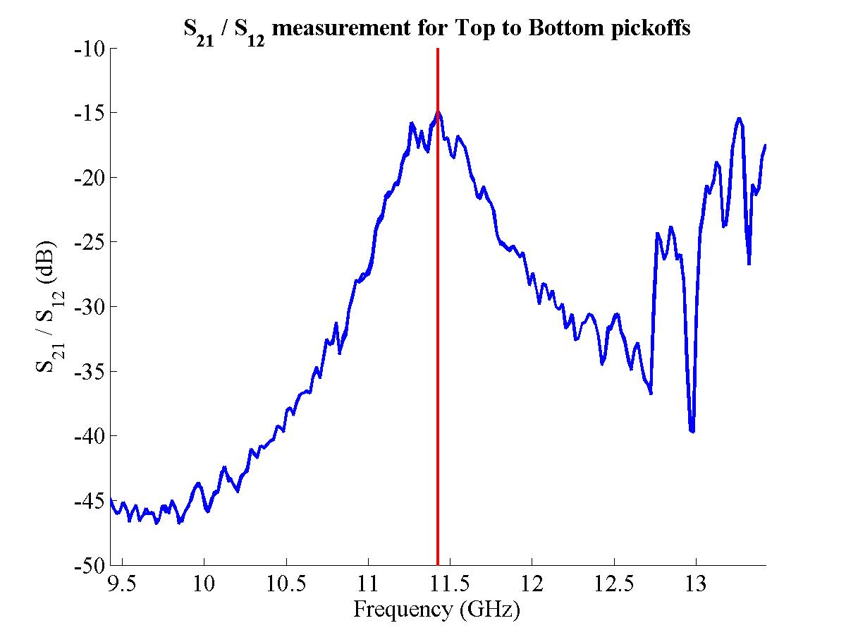
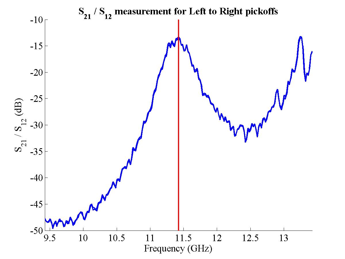
| (a) S21 for Top & Bottom | (b) S21 for Left & Right | ||||
|
|
||||
| (c) S21 for Top & Left | (d) S21 for Top & Right | ||||
|
|
||||
| (e) S21 for Bottom & Left | (f) S21 for Bottom & Right | ||||
| |||||
|
|
||||
| (a) S21 for Top & Bottom | (b) S21 for Left & Right | ||||
|
|
||||
| (c) S21 for Top & Left | (d) S21 for Top & Right | ||||
|
|
||||
| (e) S21 for Bottom & Left | (f) S21 for Bottom & Right | ||||
| |||||
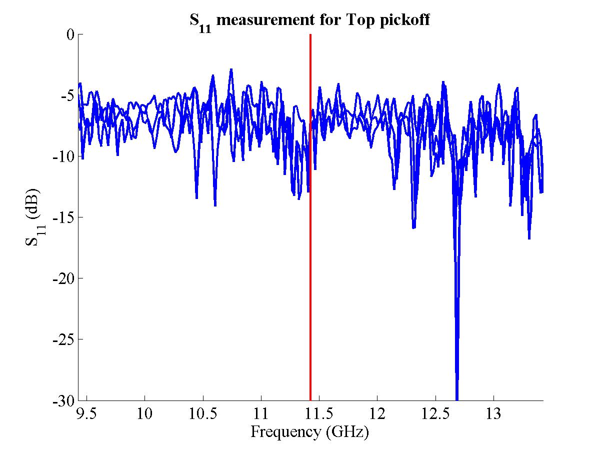
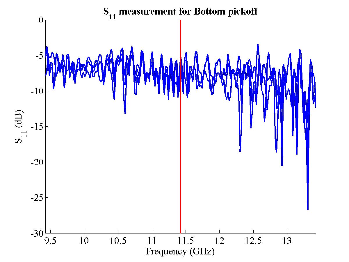
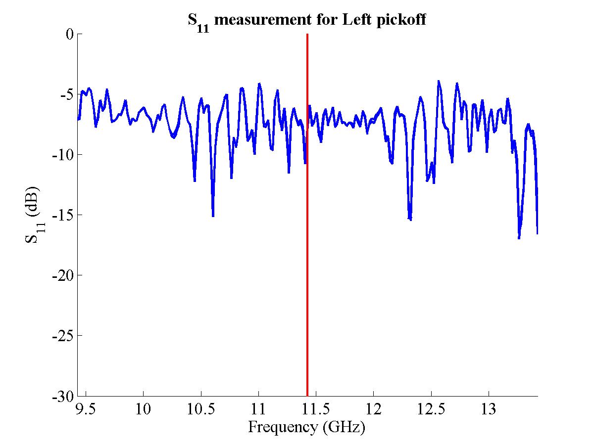
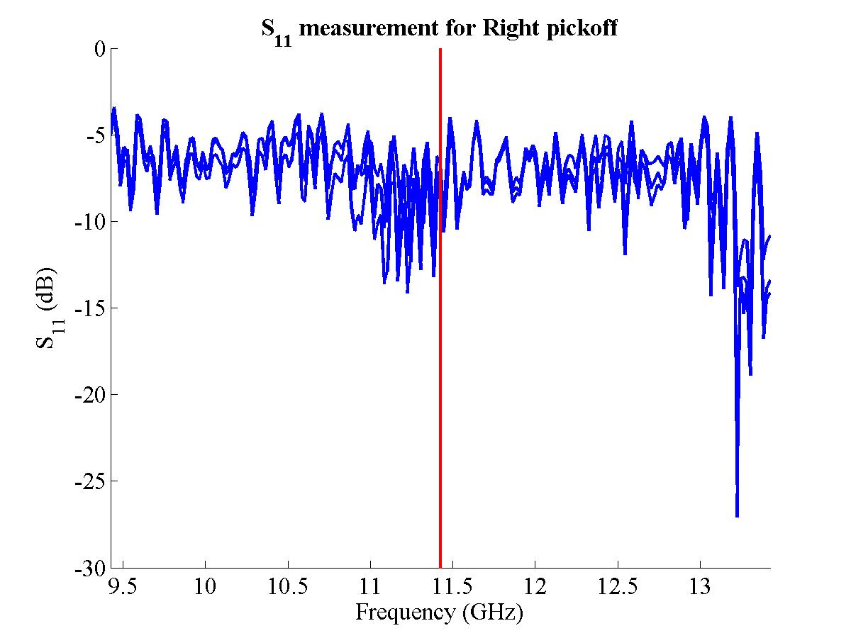
The S11 measurements for each pickoff, using the broad frequency range, are shown in Fig. 4.9. The pickoffs are named according to their position looking downstream at the BPM from the structures. The red line marks the position of 11.424 GHz on the plot. One would expect to see a trough in the reflected signal at this frequency. This is because the electrode behaves as an antenna and emits radiation mostly strongly at its resonant frequency. However, no obvious deviation from the surrounding frequencies is apparent. The likely explanation for such behaviour is that, within an enclosed cavity (such as the BPM), any RF emitted by the pickoff has nowhere to travel. Since the diameter of the beampipe is above cutoff for X-band, none can escape from the cavity: in fact, since the mode with the lowest cutoff frequency (the TE11 mode) has fc = 16.096 GHz, none of the RF within the specified range of the network analyser can escape the cavity. Therefore it is likely that, since it will be reflected within the cavity, it will be reabsorbed by the electrode. As such, any resonant behaviour of the electrode will be nullified as it absorbs the same proportion of RF as it emits for any given frequency. It is therefore likely that the S11 measurement is just a measure of the signal attenuation of the signal path between the pickoff and the network analyser.
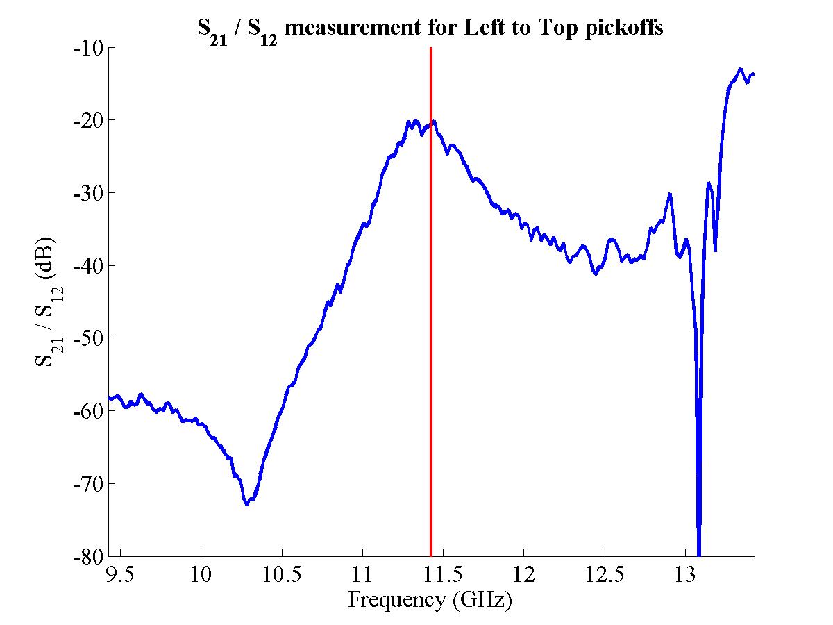
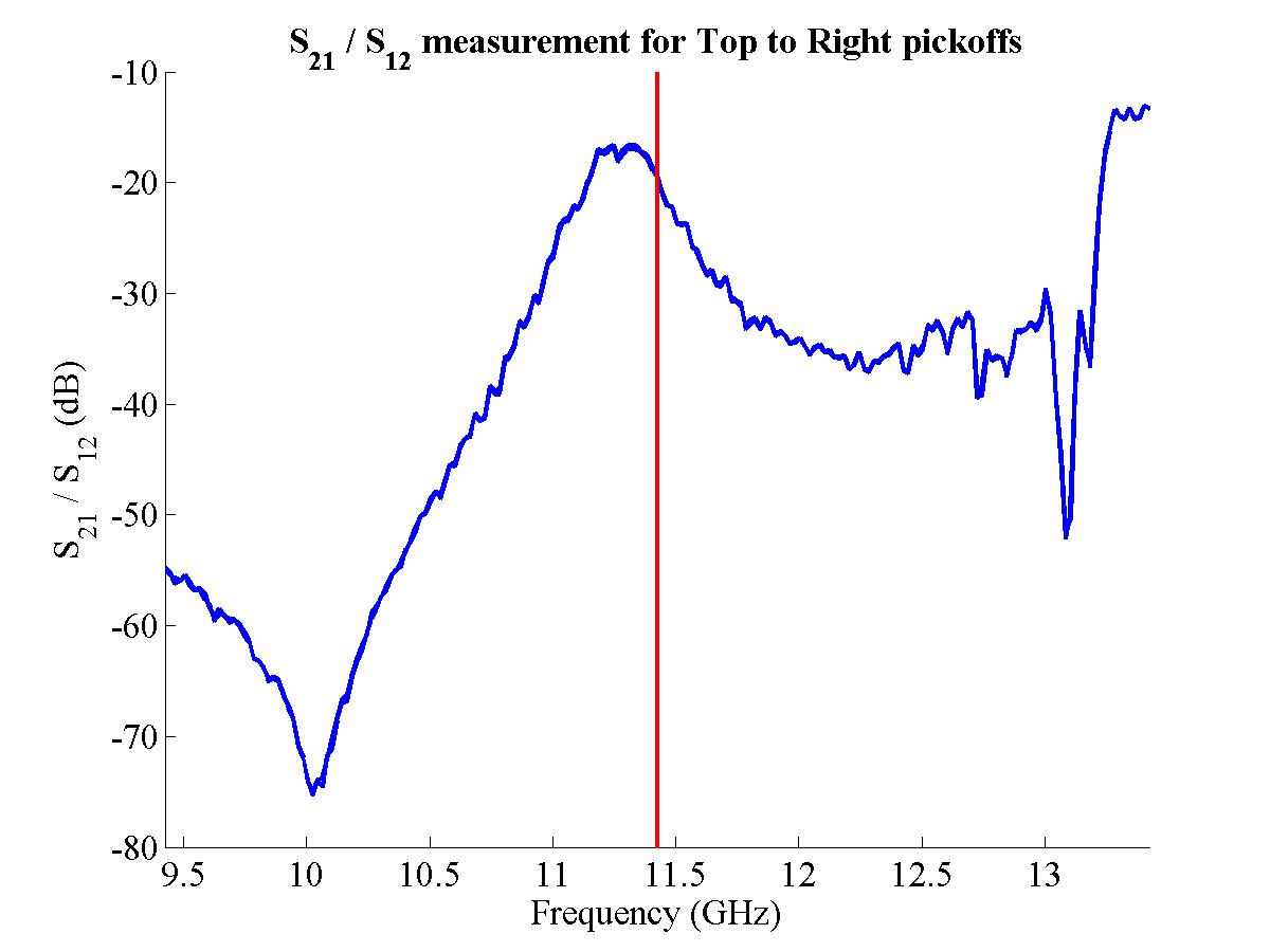
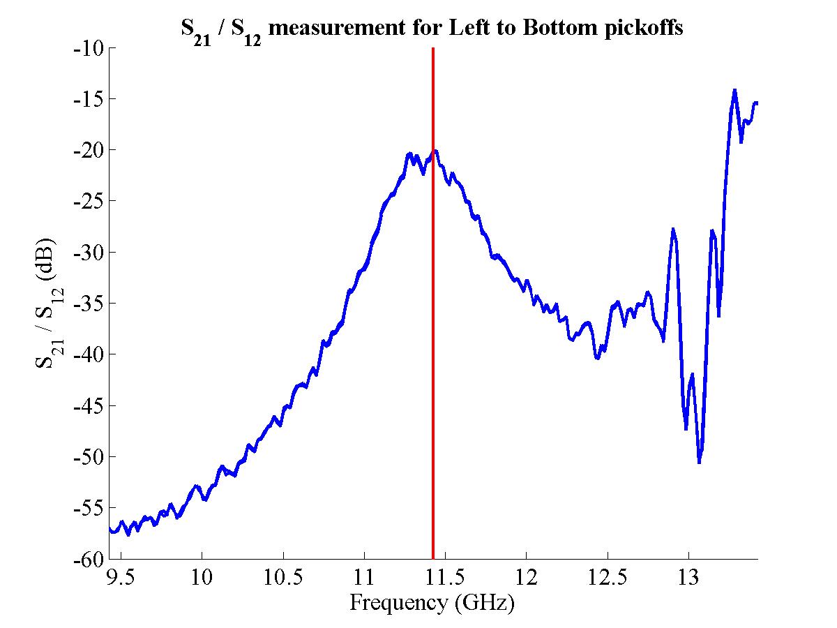
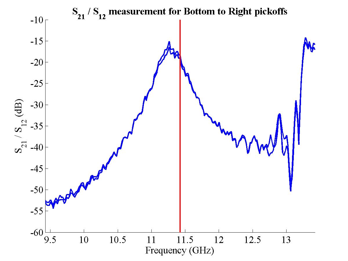
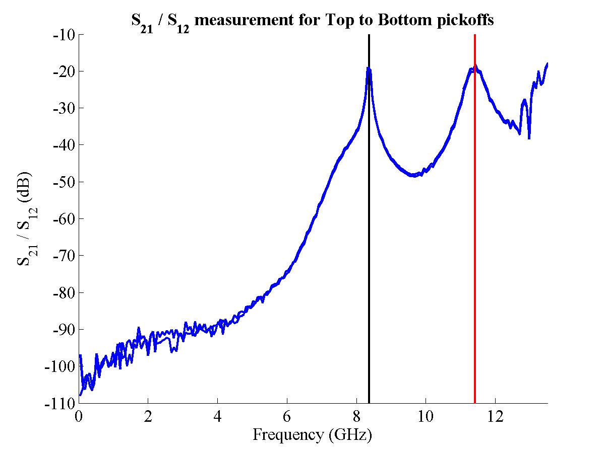
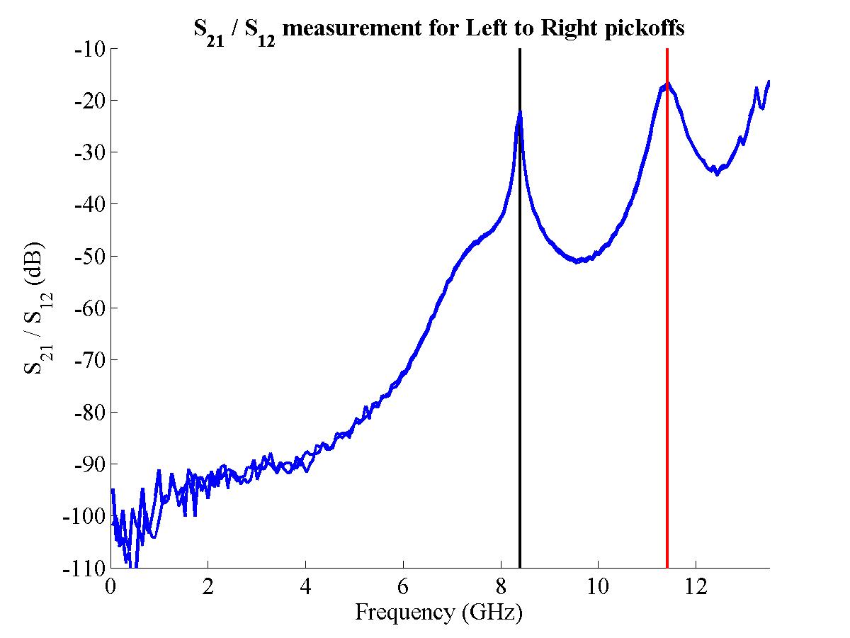
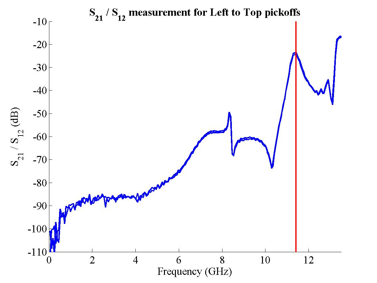
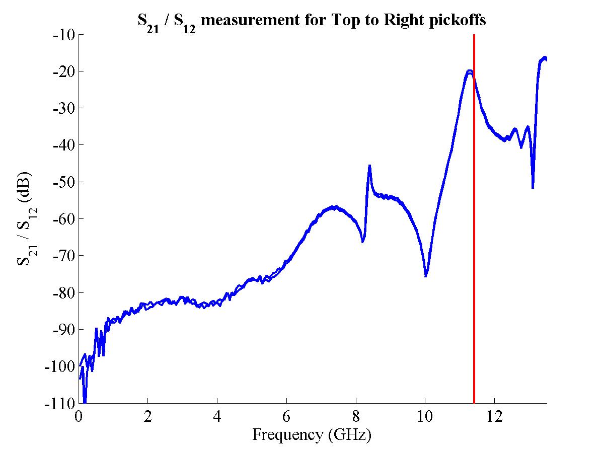
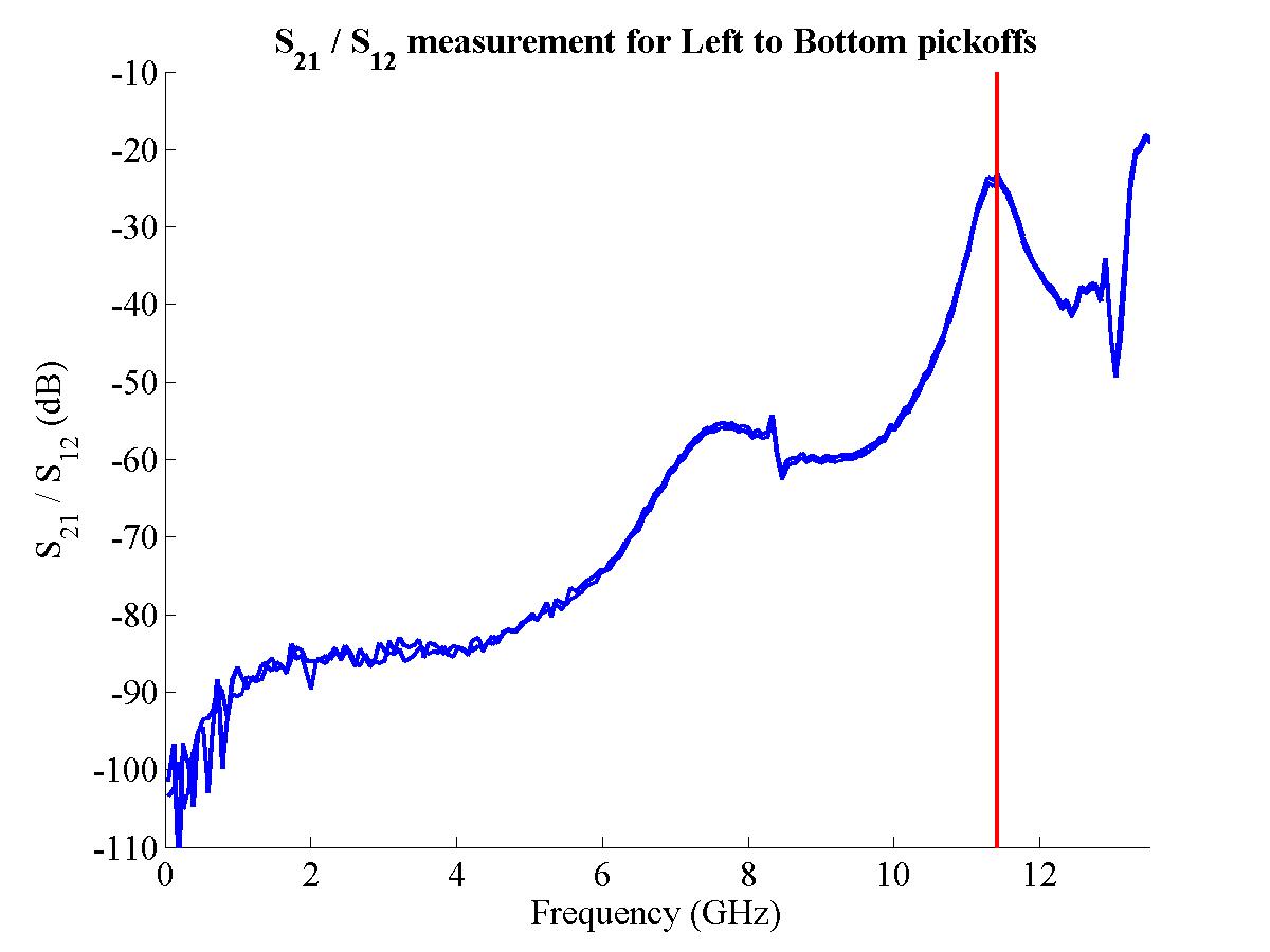
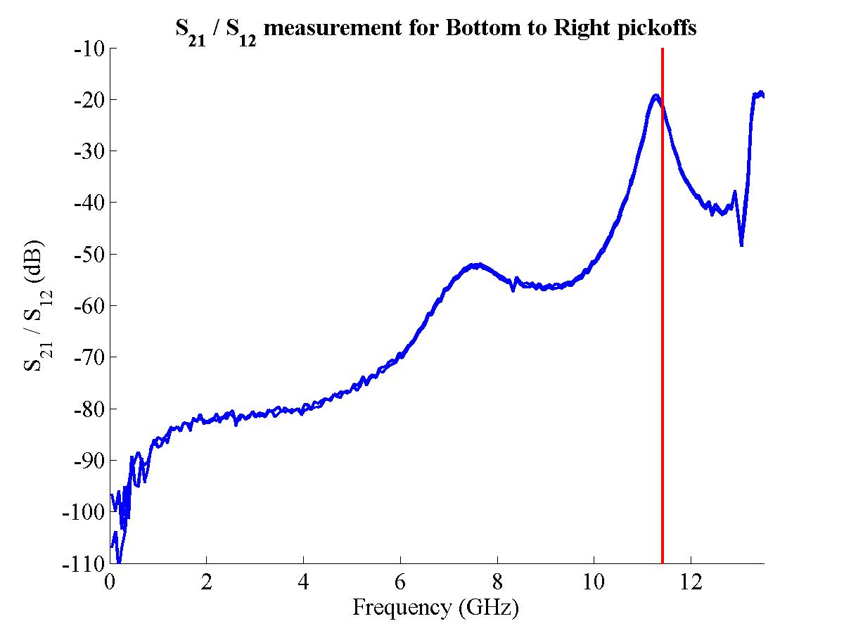
The S21 measurements do show a much clearer resonant behaviour. Fig. 4.10 shows the narrow frequency range for the S21 response for each pickoff combination, with Fig. 4.11 showing the wide frequency range. For each pickoff combination, the S21 and S12 measurements are overlaid: the almost perfect match of the two traces on each plot is an excellent confirmation of the identical transmission and reception properties of each electrode. As with the S11 measurements, the position of 11.424 GHz is marked with a red line. In each plot, a peak appears at almost exactly this frequency, indicating that each pickoff is both transmitting and receiving most strongly at X-band.
In Figs 4.11(a) and (b), which show the coupling of opposite pairs of pickoffs, a second peak also appears, at around 8.4 GHz, that is marked with a black line. It is likely that this peak corresponds to the lowest order mode within the cavity, with the frequency corresponding to a wavelength that is approximately the distance between the two electrode feedthroughs (and therefore the outer width of the spherical cube) [92]. It is approximate because the frequency of this mode is dependent on the coupling of the electrode as well as the cavity dimensions. The frequency of the peaks and the corresponding wavelength
| (4.6) |
The actual external width of the spherical cube is 35.05 mm [88]. The difference between this figure and the figures given above (as well as the difference of 0.13 mm between horizontal and vertical dimensions) is most likely due to the coupling of each antenna to the cavity.
| ||||||||||||||
|
With the S21 measurements from Fig. 4.10, it is possible to calculate the relative coupling strengths of the BPM pickoffs to the beam [56]. The S21 transmission loss at X-band, in dB, for each of the six pickoff combinations, is given in Table 4.1. The relative coupling strengths of the BPM pickoffs at X-band can be calculated from these measurements in the following way. If one denotes the signal loss between, say, the top and left pickoffs as ATL and the coupling of the top pickoff to the beam as CT, then one obtains the following set of ratios:
|
(4.7) |
|
(4.8) |
Ideally, the values for CT/CB and CR/CL should be independent of the pair of signal loss figures used in the calculation. In practice, however, a more accurate value is obtained from the S21 measurements by taking an average:
|
(4.9) |
|
(4.10) |
Using the S21 measurements given in Table 4.1 and using the fact that, since these measurements are in dB,
| (4.11) |
| (4.12) |
Converting these from dB to a raw ratio gives:
| (4.13) |
As such, there is approximately a 7% difference in coupling strengths between the top and bottom pickoffs, and a 16% difference between the left and right pickoffs. The vertical pickoffs are more closely matched than the horizontal pickoffs: since the FONT experiment will be concerned with moving and measuring a beam in just the y direction, it was the intention while constructing the BPM to maximise the performance of the vertical pickoffs, hence the better match of the top and bottom electrodes.
Finally, from these measurements it is possible to calculate the Q of the BPM. For a filter, the Q is defined as the width of the resonant peak at the −3 dB point (i.e. the point at which the frequency response has dropped by 3 dB) [62]. For the BPM measurements detailed above, one is not looking at the response of a single pickoff, but pairs of pickoffs: Q is therefore calculated from the width of the peak at the −6 dB point [43]. The following Q values for the horizontal and vertical BPM pickoff pairings are obtained using this method and calculated from the data displayed in Figs. 4.10(a) and (b):
| (4.14) |
As such, the BPM has a low enough Q (particularly in the y direction, in which the FONT experiment is most interested) to respond quickly enough to the beam to perform within the criteria given in Section 4.2, while still responding strongly at the key frequency of 11.424 GHz.
Before undertaking the more complex task of measuring beam position with the new BPM, it was necessary to measure the response of a single BPM pickoff to the beam. This would not only give an absolute scale to the measurements in the previous section (i.e. convert the relative coupling strengths of opposite pickoffs into an absolute coupling strength) but also give a measure of the filtering characteristics, time response and characteristic impedance of the BPM. To do so it was necessary to assemble a BPM processor capable of downmixing a signal at X-band.
The processor design is based upon that outlined in Section 3.3, using an RF mixer to convert the 11.424 GHz signal produced by each of the BPM pickoffs into a baseband signal. However, due to the X-band frequency used for the bunch spacing of the beam, a number of modifications were made to the initial design. The Q (given above) of the BPM would cause it to behave in a similar way to a band-pass filter at the designated resonant frequency of 11.424 GHz. In order to produce a baseband signal, one then mixes the BPM signal with a reference signal, also at 11.424 GHz, producing sum and difference. Normally one would low-pass filter the signal to remove the sum frequency, since it is only the difference frequency that is of interest. In this case however the sum frequency of 22.848 GHz is highly attenuated in most signal cabling (particularly the 3/8 in. heliax used to transmit the signal out of the NLCTA tunnel), meaning that the system as a whole behaves as a low-pass filter. More importantly, the mixers employed also did not have the bandwidth to be able to output a signal of such high frequency.
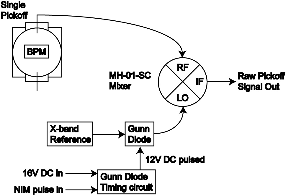
A block diagram of the components for the first BPM processor is shown in Fig. 4.12. The signal from each pickoff was connected, via a length of SMA cable, to the RF input of a Pulsar Microwave
| Figure 4.12: Block diagram showing the X-band BPM processor used for the single pickoff BPM measurements. A second mixer is used for the other pickoff. |
The intention, as with the IPFB BPM processor, was to downmix the pickoff signal to baseband and transfer this downmixed signal to a DAQ system outside the tunnel. The IF port of each mixer was connected to a 35 m long piece of 3/8 in. heliax cable which was used to carry the signal from the tunnel; a Tektronix digitising oscilloscope recorded each of these pickoff signals. An initial problem occurred in finding an appropriate signal for the mixer LO input. The LO input required for the
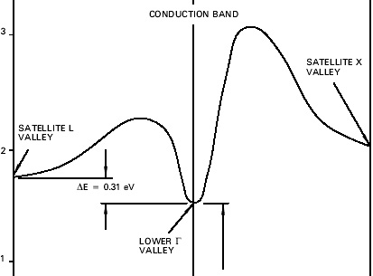
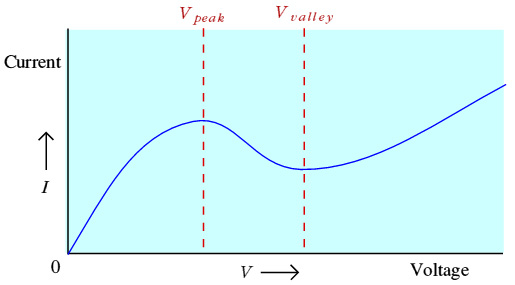
A Gunn Diode is a microwave oscillator that takes advantage of the Gunn Effect within a semiconductor (usually GaAs). The Gunn Effect is a result of the band structure that exists within particular semiconductors; examples are shown for the Gallium Arsenide (GaAs) semiconductor most commonly used for Gunn diodes [94]. Fig. 4.13(a) shows the conduction band within GaAs. With a low applied field (i.e. small potential difference) the electrons within the semiconductor reside within the central valley (Γ) of the conduction band. Within this region the semiconductor has a linear I-V relationship. Once the applied field reaches a certain threshold value (Vpeak, as marked in Fig. 4.13(b)), electrons begin to gain enough energy to populate the satellite valley (L). Within this valley the electron mobility μ is considerably lower, with a much larger effective mass: this splitting of the electrons between energy levels causes the semiconductor to behave nonlinearly (see below). Once all the electrons have acquired sufficient energy to populate the satellite valley, the semiconductor takes on the I-V characteristics of this higher energy state and recovers its linear behaviour.
|
|
||||
| (a) GaAs conduction band [94] | (b) GaAs I/V curve [95] | ||||
|
|||||
While the applied voltage is between Vpeak and Vvalley, as shown in Fig. 4.13(b), the semiconductor exhibits distinctly nonlinear behaviour34. This behaviour is due to the superposition of the markedly different I-V characteristics, resulting from the large difference in effective electron mass, of the two valleys within the conduction band. This gives the Negative Differential Resistance (NDR) behaviour shown in Fig. 4.13(b) where, between Vpeak and Vvalley, dI/dV becomes negative. It is this negative differential resistance (usually termed just negative resistance) that is harnessed by the Gunn Diode [95].
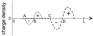
| Figure 4.14: Creation of a Gunn domain within n-doped GaAs [94]. Charge perturbation between A and B causes a net positive charge distribution, giving rise to an initial Gunn domain (solid line); this increases with time as it travels towards the anode (dashed line). The horizontal axis indicates the direction of majority carrier flow for a strip of length L. |
In order to create a Gunn diode, a strip of n-doped GaAs is biased with a voltage V such that
By AC coupling the signal at the anode it is possible to create a microwave frequency RF signal: this device is known as a Gunn diode. The signal is usually tuned and enhanced by placing the Gunn diode within a resonant coaxial cavity, the dimensions of which set the output frequency of the diode [95]. Tuning the output frequency is achieved by inserting a rod into the resonant cavity to adjust the resonant frequency; a screw is used to retract the rod from the cavity and change the resonant frequency [96]. It is also possible to drive the cavity at a particular frequency, causing it to resonate with a desired RF signal and behave as an RF amplifier. In addition, running the Gunn diode with a pulsed voltage bias can produce a higher output power. Heat dissipation is important for the diode as a high temperature, resulting from poor heat dissipation, can cause breakdown within the bulk semiconductor. Pulsing the voltage allows higher peak output powers to be reached without damaging the diode.
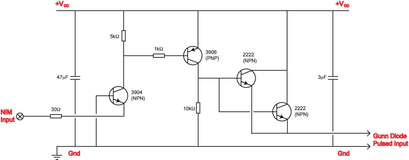
The Gunn diode used for the X-band BPM mixer LO input was a Microwave Device Technology MO86651-M02 X-band oscillator. The diode is designed to be operated by a pulsed 12 V signal: to provide this signal a separate circuit, designed by Josef Frisch, was assembled. The circuit diagram for this circuit is shown in Fig. 4.15. This circuit requires two inputs: a NIM trigger input and a ~16 V DC power supply input. This DC input was adjusted to set the output pulse to exactly 12 V, since the Gunn diode is very sensitive to variations in this voltage pulse: too low and the output power begins to drop rapidly; too high and the diode starts to draw a large amount of current, causing it to overheat [30]. The switching action of the 3904 transistor allows current to flow through the 3906 transistor in time with the NIM pulse. The 3906 in turn switches on the pair of 2222 transistors which provide the 12 V pulses for the Gunn diode.
| Figure 4.15: The timing circuit used to supply the +12 V pulse to power the Gunn diode. The circuit takes a ~16 V DC input, plus a NIM input that provides the timing and pulse shape. |
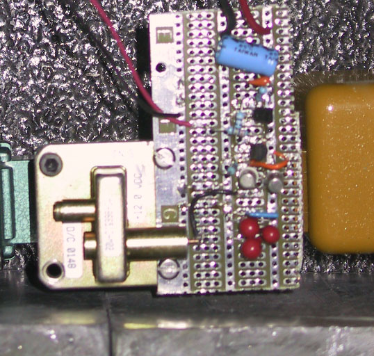
| Figure 4.16: The Gunn diode mounted to its timing circuit: the adjustment screw is mounted on the left hand side of the waveguide assembly. |
This timing circuit was mounted onto the back of the Gunn diode waveguide assembly: this is shown in Fig. 4.16. The main chassis of the diode was used as the ground, with the output of the timing circuit connected to the input pin of the diode itself. The two input signals (NIM and +16 V DC) for the timing circuit were carried on two coaxial cables into the NLCTA tunnel. The Gunn diode was initially designed to be used on its own to provide the X-band reference signal for the X-band BPM mixers. However it was not possible to check that the Gunn diode would be phase locked to the beam signal; nor was it possible to set the output frequency to exactly 11.424 GHz. The Gunn diode signal path was therefore modified slightly to allow an external signal to cause it to lock to the beam phase and frequency. This was achieved by driving the Gunn diode with the X-band reference signal from the NLCTA RF system, as mentioned above (see Fig. 4.12). The reference input causes the resonant cavity of the Gunn diode to oscillate at a particular frequency — in this case 11.424 GHz — exciting the diode to resonate at this frequency.
| Figure 4.17: The Gunn diode with its timing circuit attached, and mounted to a waveguide T connector. The two isolators to the left and right of the Gunn diode carry power in from the reference signal to phase lock the diode output (grey), and out from the diode to the BPM mixers (yellow). The two cables appearing from the top are the NIM trigger input (left) and timing circuit 16 V power supply. |
This reference signal input was assembled from a pair of RF isolators, attached to a waveguide T connector: the experimental setup is shown in Fig. 4.17. An isolator is a device that allows RF power to pass through it one only one direction35. One isolator allowed the X-band reference signal to pass into the Gunn diode, while preventing any reflections from the diode from interfering with the reference signal input. A second isolator allowed the output of the Gunn diode to pass onto the mixer LO ports, while preventing any RF from reflecting back into the Gunn diode and disrupting the phase locking. The output of the second isolator was then connected to a 4-way splitter to allow distribution to the two mixers; a third output of the splitter was connected to another heliax cable to allow measurement of the Gunn diode output outside the tunnel, with the fourth output terminated with a 50 Ω terminator.
|
|
||||
| (a) Power Output | (b) Phase lock | ||||
|
|||||
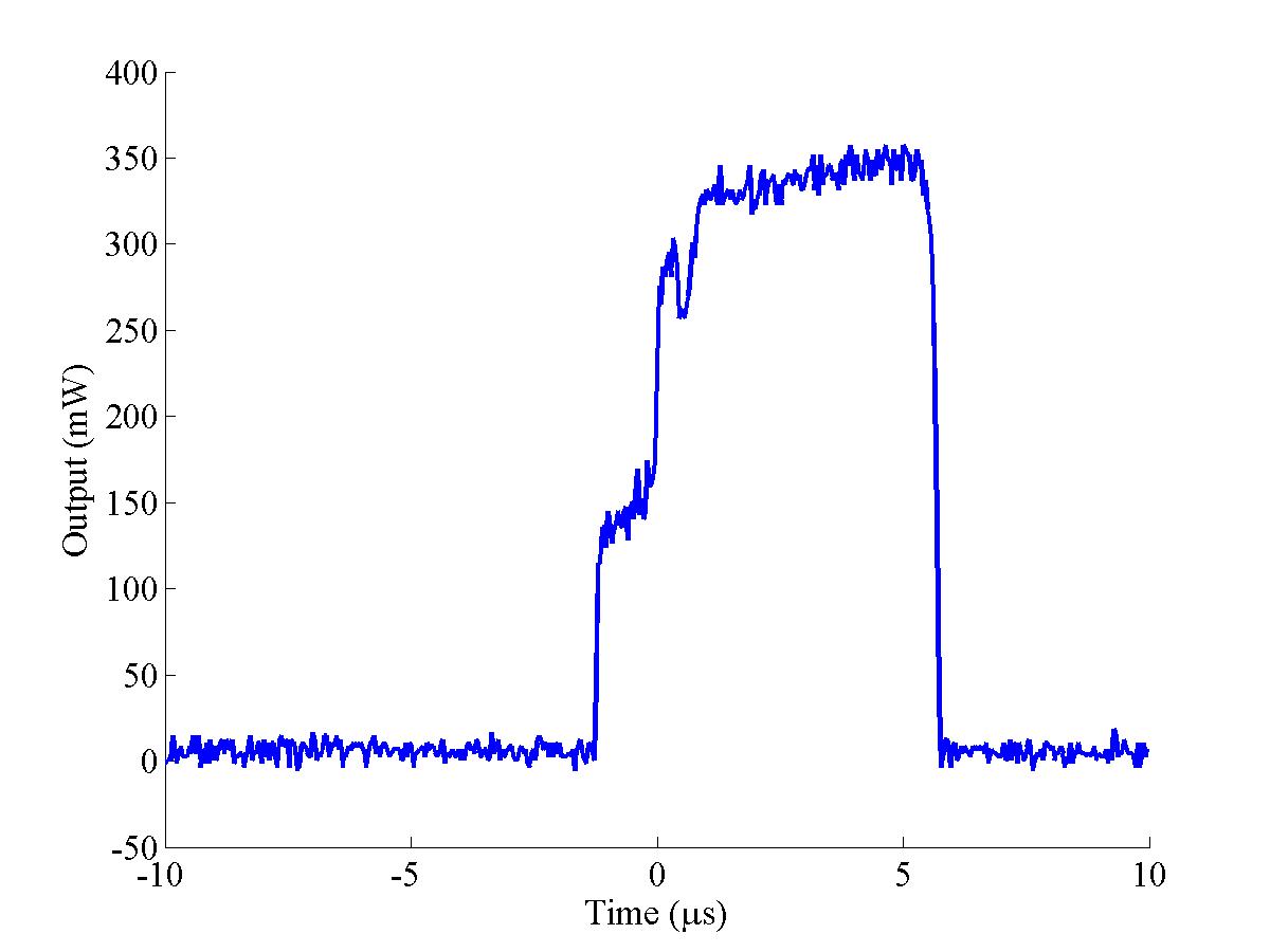
The output power of the Gunn diode is shown in Fig. 4.18(a): at the rear end plateau of the pulse, this is
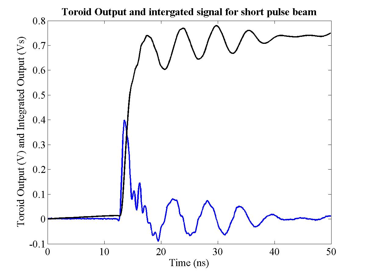
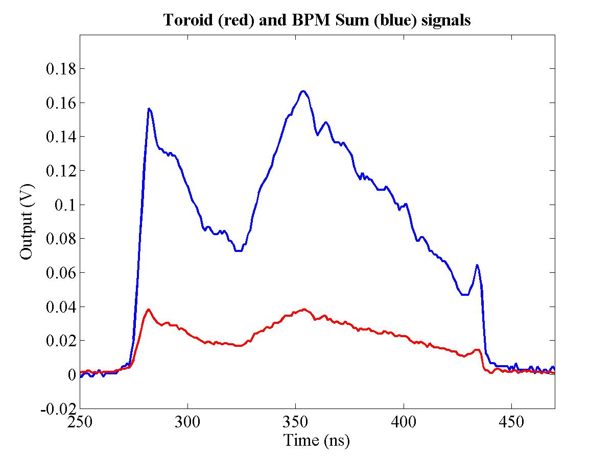
Having constructed a processor to process the signal from a single pickoff, the response of that pickoff could now be tested. The top pickoff was connected to the mixer RF port (as shown in Fig. 4.12), with the other three unused pickoffs terminated. In order to provide a corroborative signal and a measure of the beam charge, the output of the toroid that resides between the the BPM and QD1760 (TORO 1750 — see Fig. 4.8) was also recorded. A Toroid (also known as a “beam transformer”) is essentially a coil of wire wrapped around a ferromagnetic core that is mounted around a ceramic insert in the beampipe [97]. The ceramic insert allows the EM-field surrounding the beam to penetrate the beampipe. The toroid converts the passing beam current signal into a voltage that can be measured: TORO 1750 produces an output of approximately 1.25 V per Amp of beam current [98].
While normally connected to the NLCTA DAQ system, for the X-band BPM tests the output of TORO 1750 was connected to the scope that was used to record the X-band BPM pickoff signals. This scope in turn was connected, via GPIB, to a PC running Matlab inside the NLCTA Control Room, to allow acquisition and storage of the various BPM and toroid signals. For this first series of single pickoff tests, the NLCTA was run in short pulse mode (see Table 3.3). By changing the NLCTA gun it was possible to alternate between the short and long pulse sources, providing either a ~2 ns or ~170 ns pulse. To measure the impulse response of a single BPM pickoff, the short pulse source was used. This would allow a measure of the coupling strength and time response of the BPM.
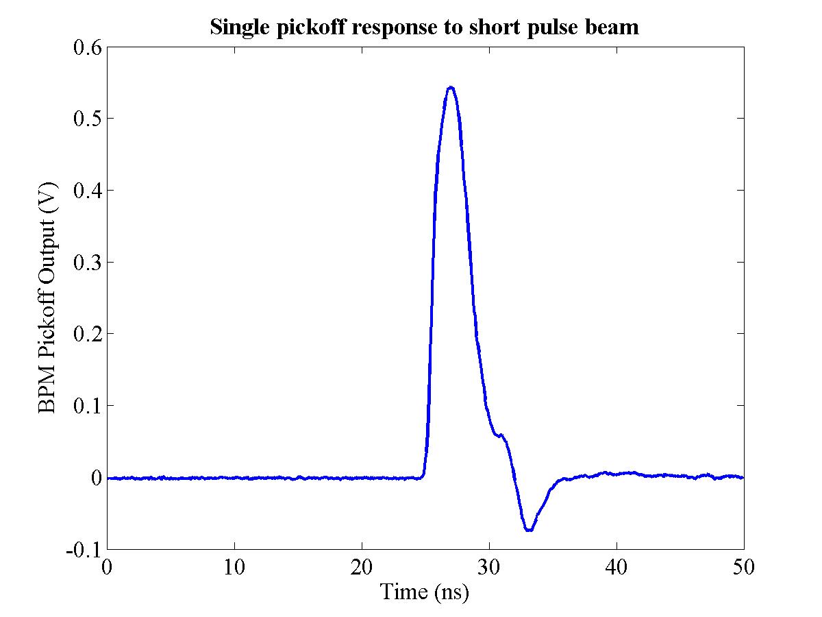
| Figure 4.19: Response of a single BPM pickoff to the short pulse beam; the plot shows the average of 5 pulses. |
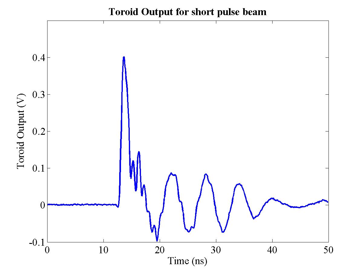
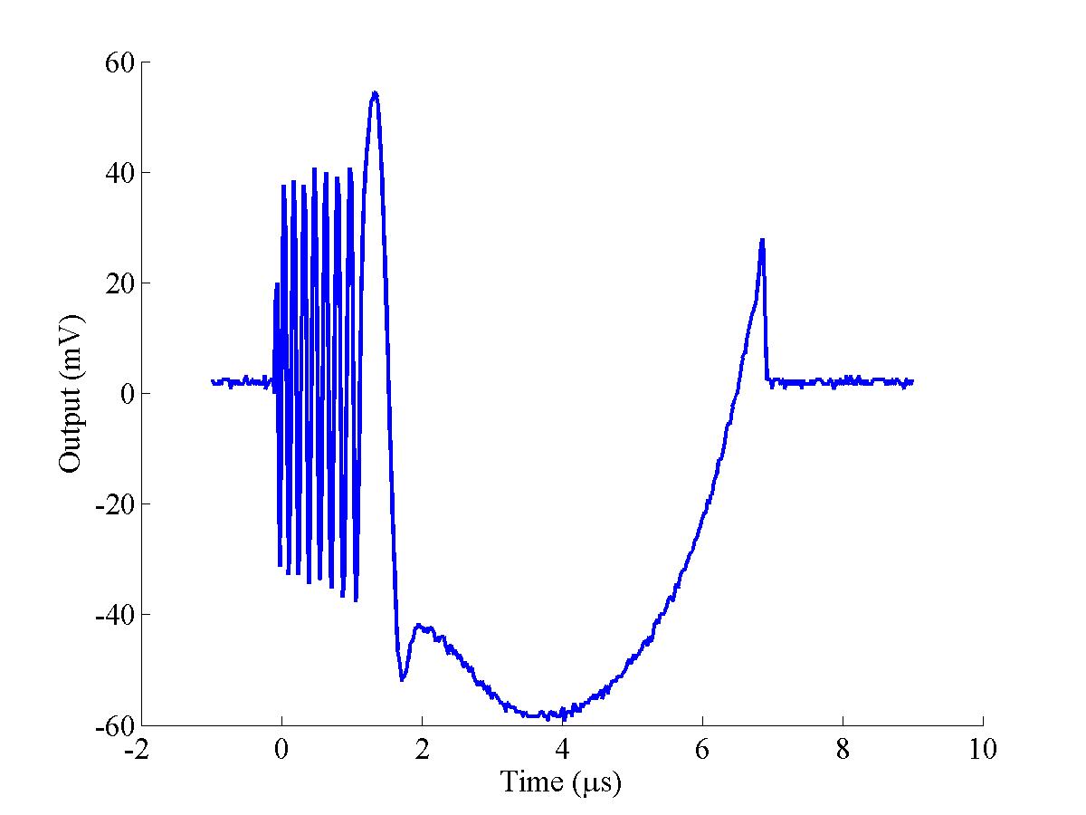
| Figure 4.20: Toroid output for short pulse beam; the plot shows the average of 5 pulses. |
The output of a single BPM pickoff in response to the short pulse beam is shown in Fig. 4.19, with the corresponding toroid output shown in Fig. 4.20; each of these plots is the average of 5 beam pulses. At first glance it is encouraging to see that the BPM pulse tracks the output of the toroid, but with less of the noise that appears on the falling edge of the pulse. However, some features do appear on the BPM pulse: these are discussed in more detail in Section 4.5.2. The coupling strength of the BPM to the beam is defined as the output in volts of the pickoff per amp of beam current. Since this is essentially V/I, the coupling strength of the BPM can also be expressed as a characteristic impedance, ZBPM:
| (4.15) |
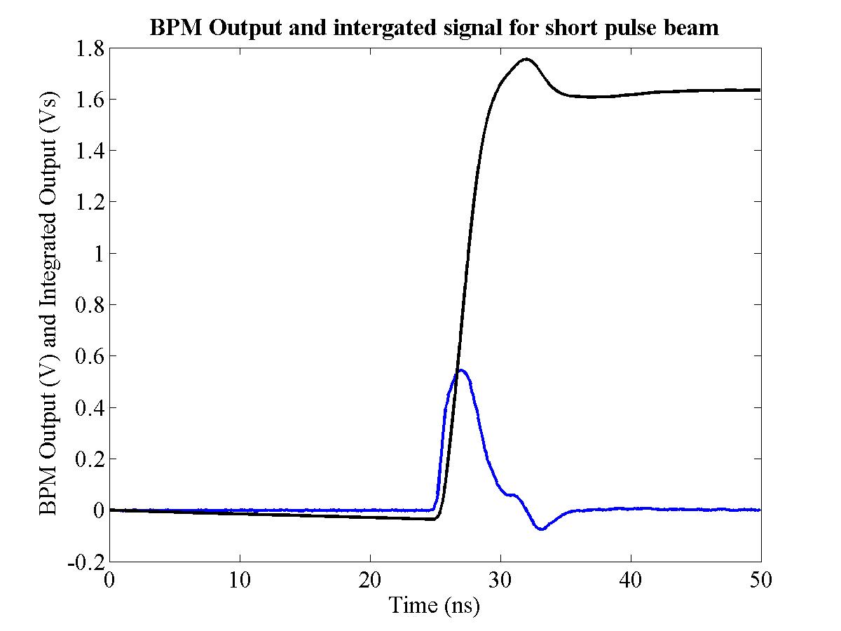
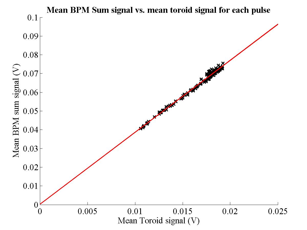
To calculate the characteristic impedance of the BPM it is necessary to compare the voltage output of the BPM pickoff to the actual beam current. The current measurement is provided by TORO 1750: since there are no beamline components between the X-band BPM and the toroid, it is acceptable to assume that the current measured by the toroid is the same as that passing through the BPM. However, in order to account for the features that appear on the falling edge of both signals, the integral of both signals must be used for this comparison: the integrated signal gives an output in Volt-seconds that is independent of the response time of the apparatus in question; all that is important is that the signal has settled to a suitable degree. From these integrated signals, the total bunch charge and BPM coupling strength can be calculated. The integrated toroid output, in Amp-seconds (Coulombs), is given by:
| (4.16) |
for a pulse of length (t2 − t1), toroid voltage Vt at time t, data sampling interval of Δt and toroid beam coupling strength of 1.25 V/A. The corresponding equation for the BPM, in Volt-seconds, is:
| (4.17) |
for BPM voltage Vt at time t. Therefore the result of Eq. (4.17) divided by Eq. (4.16) gives the characteristic impedance of the BPM in Ohms. The integral of the BPM and toroid signal outputs is shown in Figs. 4.21 and 4.22 overlaid with the original signal pulse. From this integrated pulse, a preliminary coupling strength for the single pickoff in question can be calculated. In both cases, the integrated pulse at 45 ns was chosen to have reached a suitable level of stability [30]. The data from two separate runs was used: the integrated voltage output for both toroid and X-band BPM is shown in Table 4.2. The average of the two coupling values gives an initial value of ZBPM = 2.77 Ω.
| ||||||||||||||
| ||||||||||||||
| Figure 4.21: Integrated BPM signal for short pulse beam. The raw BPM pickoff signal is shown in blue, with the integral of that signal shown in black. |
| Figure 4.22: Integrated toroid signal for short pulse beam. The raw toroid signal is shown in blue, with the integral of that signal shown in black. |
However, having calculated an initial coupling strength, one must take into account the attenuation of all the components in the BPM signal path to be able to accurately measure the coupling of the BPM proper to the beam. As such, a number of measurements were made using the components that sit in the signal path between the BPM and the scope for data taking. The signal loss for each component was calculated using the same
| ||||||||||||
|
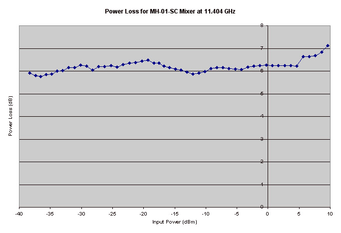
An output frequency of 11.404 GHz was chosen for the RF signal generator for the RF input to the mixer, as it close enough to 11.424 GHz while still providing a measurable 20 MHz IF frequency. The components between the BPM and the mixer are listed in Table 4.3, in order from BPM SMA output to mixer RF input, along with the measured signal loss for each component. The mixer signal loss as a function of RF input power is shown in Fig. 4.23. The average signal loss for the central power range is 6.15 dB: this gives a total signal loss from X-band BPM to mixer of 21.84 dB.
|
Figure 4.23: Signal loss for the |
The signal from the mixer used in the BPM processor to the scope is carried on a 3/8 in. heliax cable that is 100 m in length. Having been downmixed by the processor, the BPM signal is no longer predominantly at 11.424 GHz, but a DC signal approximating the beam pulse envelope. The short pulse of ~4 ns, as seen in Figs. 4.19 to 4.22, corresponds to a frequency of ~250 MHz; at this frequency, the entire heliax cable assembly — consisting of an SMA to N-type adapter, the heliax cable, an N-type to BNC adapter and ~2 m of BNC cable connected to the scope — was measured to have a total attenuation of 3.90 dB. This gives a total signal attenuation — from BPM to scope — of 25.75 dB. This attenuation reduces the output signal power of the BPM pickoff by a factor of 375.6; this corresponds to a reduction in voltage by a factor of 19.4.36
The true voltage output of the BPM pickoff is therefore 2.77×19.4 = 53.8 V/A, giving the top BPM pickoff a characteristic impedance of ZBPM = 53.8 Ω. Using the coupling ratios calculated in Section 4.3.3, Eq. (4.13), it is possible to calculate the coupling strength of both vertical pickoffs:
| (4.18) |
These values compare favourably to the coupling strength originally predicted for the BPM of 40 Ω [30]. It is also an interesting coincidence that the measured coupling strength is very close to the transmission line impedance of 50 Ω.
The second parameter required to characterise the BPM is its time response; this is also possible to determine from the data shown in Fig. 4.19. The time response of the BPM is defined in terms of the associated decay constant in the same manner as a discharging RC-circuit: it was therefore assumed that the BPM behaved in the same fashion as an RC-filter circuit, with an associated RC decay constant (commonly RC or τ, with units of seconds). Functionally, this RC time constant is the time it takes for the output of a discharging RC circuit to reach 1/e (or 0.37) of its initial value [62]. The differential equation governing the behaviour of such a circuit is:
| (4.19) |
where Vi is the circuit input voltage, Vo is the output voltage, and both are functions of time. To obtain Vo as a function of Vi, the solution to Eq. (4.19) is:
| (4.20) |
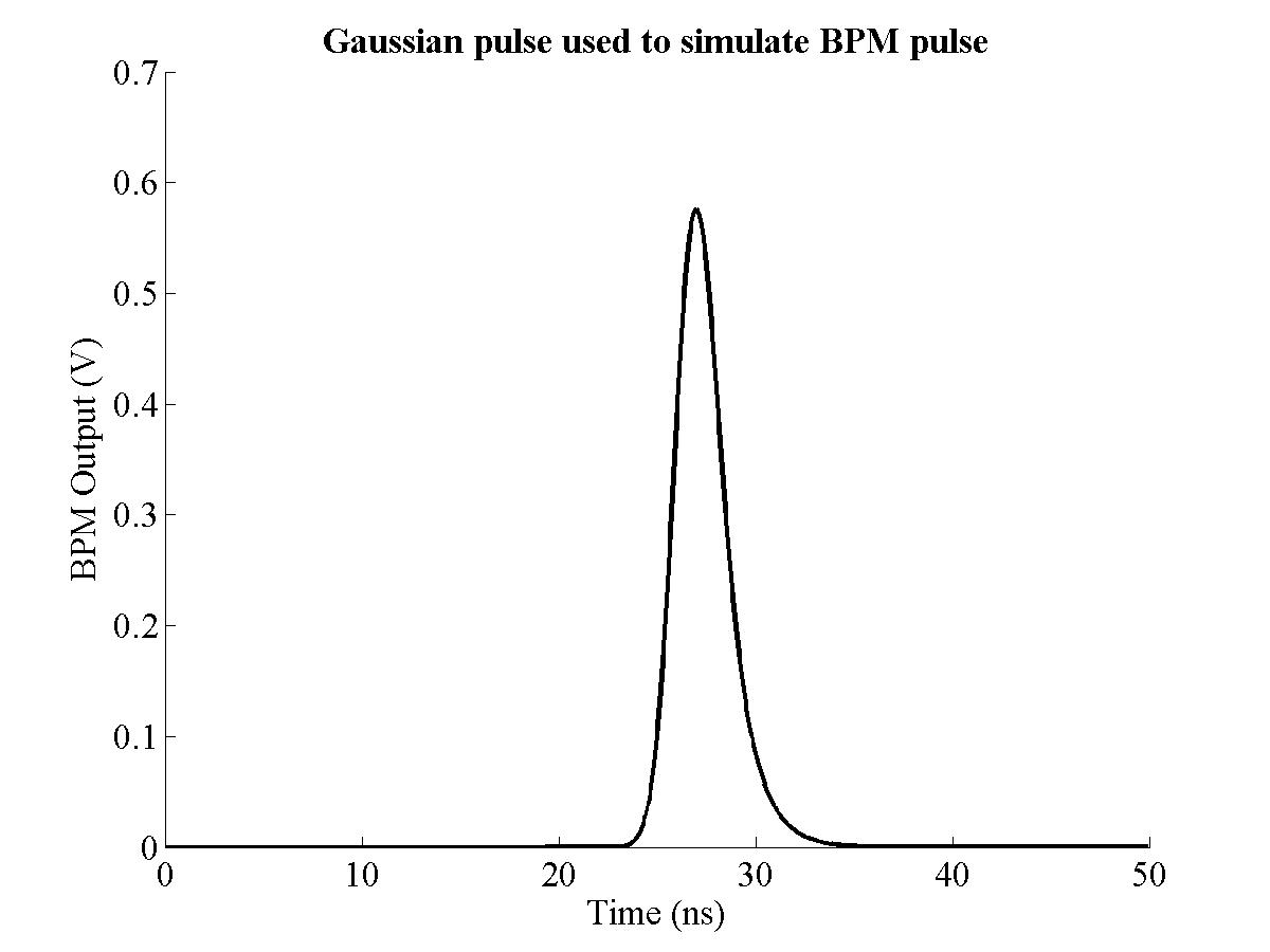
where τ is a dummy variable for the purposes of integration [62]. The next stage is to accurately model the pulse shape of the incoming beam. The initial assumption was that the charge distribution along the length of the bunch train was approximately Gaussian. This essentially means that the time structure of the beam — Vi(τ) in Eq. (4.20) — has the following shape:
| (4.21) |
where σ is the standard deviation of the charge distribution along the length of the bunch, A is a scale factor and t0 is the time corresponding to the centre of the pulse (the mean position). The usual 1/(σ√) scale factor is here absorbed into A, since A will be scaled to the size of the beam and so incorporates all such scale factors. All units within the exponential are in nanoseconds; A has the units of Volts. The integrand in Eq. (4.20) therefore becomes:
| (4.22) |
where one has now incorporated all of the scale factors into the single constant A. The lower limit is chosen as −20 to allow the integration to be solved numerically: at this point the function is negligibly close to zero. This numerical integration was carried out by the program Maple, giving the following result:
| (4.23) |
where erf is the error function [99]; erf(x) is twice the integral of the Gaussian distribution with mean 0 and variance of 1/2:
|
Having found the functional form of this RC-filtered Gaussian, the next step is to fit this Gaussian with its 4 independent parameters — RC time constant, t0, σ and A — to the data: this was accomplished in Matlab using the fminsearch function. fminsearch takes an input function and, by varying any number of specified input parameters (constants upon which the function is dependent), finds the minimum of that function. In this case, the function to be minimised is a χ2: this is calculated using the data points for the recorded BPM data (such as that shown in Fig. 4.19) and those generated using Eq. (4.23) with the fitted parameters for discrete time intervals. Minimising the χ2 of these two curves involves varying the four input parameters until χ2 reaches a minimum value. For the purposes of the fit, the χ2 was defined in the following way:
| (4.24) |
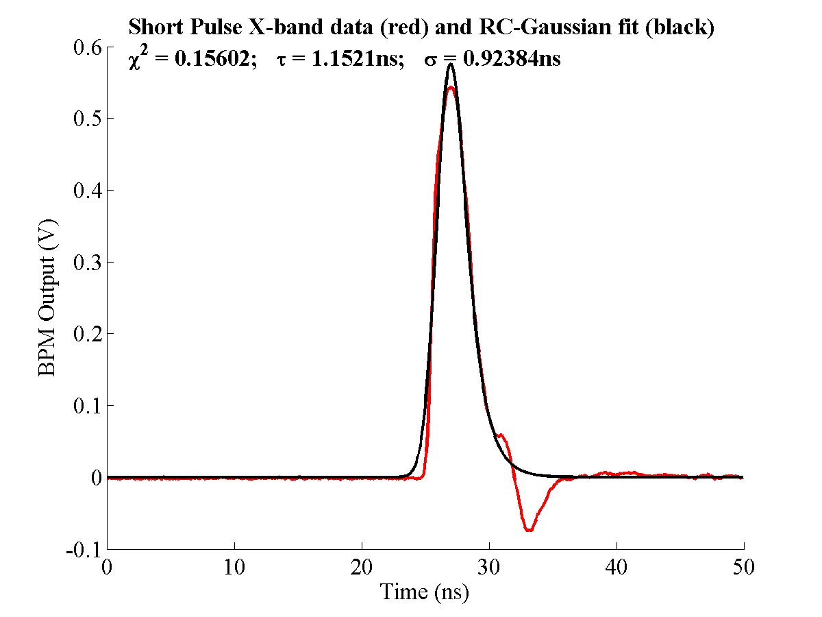
for k data points yi and fitted function Vo(t) at discrete time ti. For an RC-filtered Gaussian function the fit for one dataset is shown in Fig. 4.24.
| Figure 4.24: RC-filtered Gaussian pulse fitted to raw BPM pickoff data for short pulse beam. |
Fig. 4.24 uses the same raw data shown in Fig. 4.19. Two of the fitted values (RC and σ) are shown on the plot: since one is no longer dealing with a real RC circuit but with raw time constants, RC is given as τ. It is a measure of the validity of the χ2 fit that the value of τ produced by fminsearch is around a nanosecond, as one would expect from the width of the pulse.
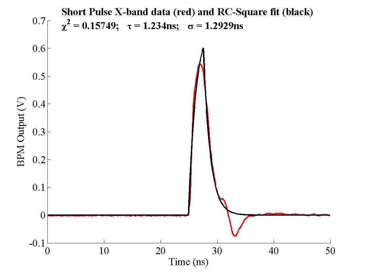
It is also possible to model the bunch train as a square pulse. Although functionally this is more complex due to the discontinuities inherent in a step function, it becomes very simple analytically if one splits the modelled response into 3 parts. If one assumes that the bunch train has a uniform charge distribution and passes through the X-band BPM between time t1 and t2, then prior to t1 the response of the BPM is necessarily zero. Between t1 and t2 the response has the form:
| (4.25) |
Eq. (4.25) describes an exponential decay from zero towards the value A: in the case of the BPM pulse fit A is the peak or plateau value of the step function. After time t2, the response becomes:
| (4.26) |
Eq. (4.26) describes an exponential decay towards zero from a value
| Figure 4.25: RC-filtered square pulse fitted to raw BPM pickoff data for short pulse beam. |
Although the fit for the leading edge of the pulse is better than that for a Gaussian pulse, this is offset by the poor fit for the falling edge, resulting in a larger time constant τ. However one can again see that the fitting process produces results of the correct order of magnitude, since τ, at 1.234 ns, is only ~15% larger for the square pulse than the Gaussian fit. It is therefore a plausible deduction that the BPM behaves with characteristics similar to that of an RC circuit, with a time constant on the order of 1.2 ns.
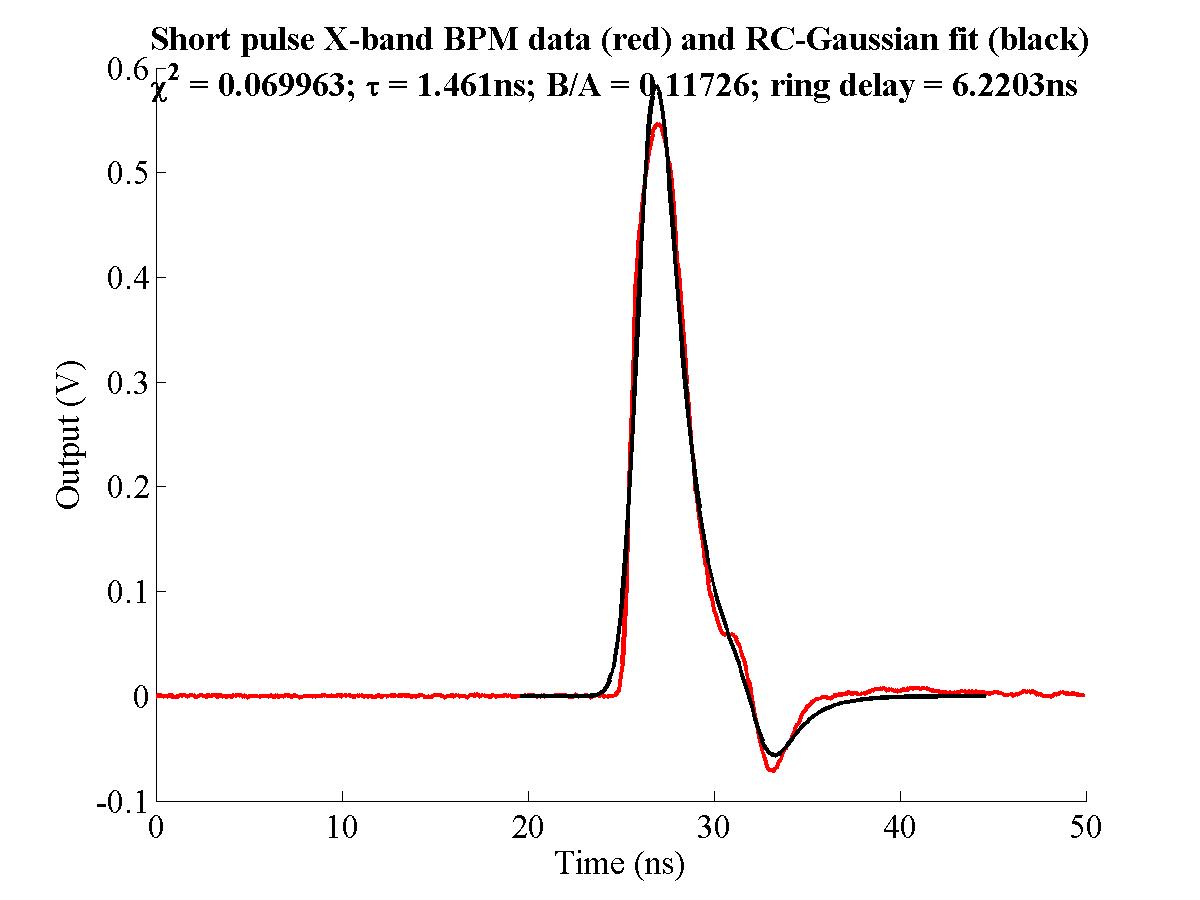
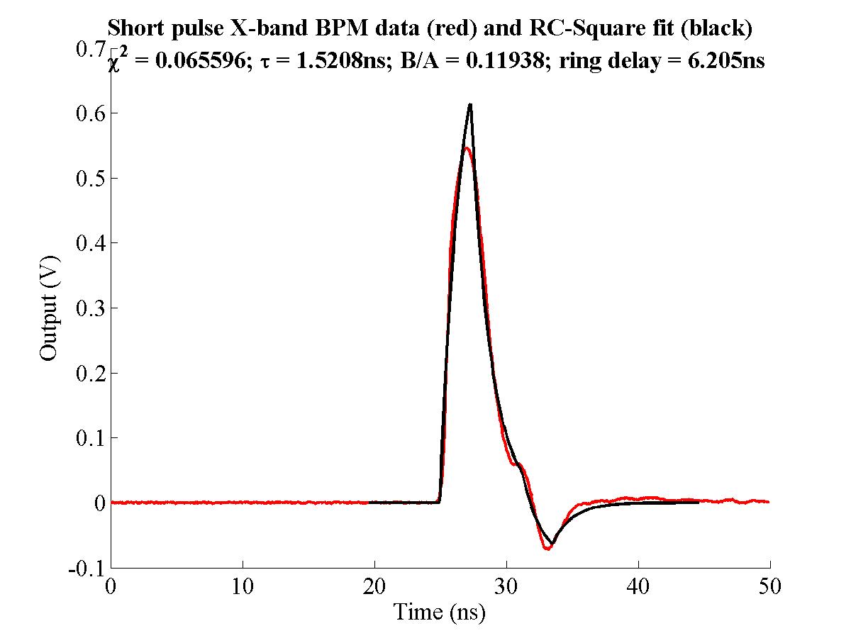
An improved fitting procedure was written by Gavin Nesom in an attempt to characterise the ringing that appears at around 33 ns [100]. The hypothesis was that this ringing was caused by a signal reflection from one part of the processor circuit, which would then travel back to the BPM pickoff, reflect off the pickoff, invert and follow the original signal with a measurable time delay. The fitting routine using fminsearch was modified to model the reflection by inverting, shrinking and delaying the original signal and adding it to the original. The number of fitted parameters was expanded to six to include the magnitude of the reflection (denoted by B) and the time delay between the original BPM signal and the reflected signal, tr. A necessary boundary condition on the fit was that the previous fit parameters of τ and σ are the same for the reflection as the original signal. Both beam models — of RC-filtered Gaussian and square pulses — were used for this improved reflection model.
| Figure 4.26: RC-filtered Gaussian pulse with signal reflection fitted to raw BPM pickoff data for short pulse beam. The number B/A gives the ratio of the magnitudes of the primary pulse to the reflected pulse. |
| Figure 4.27: RC-filtered Square pulse with signal reflection fitted to raw BPM pickoff data for short pulse beam. The number B/A gives the ratio of the magnitudes of the primary pulse to the reflected pulse. |
The results for each fitting method are shown in Figs. 4.26 and 4.27, with various fitted parameters shown in Table 4.437, including the ratio of the magnitudes of the reflected signal to the original signal, B/A. The first point to note is that the quality of the fit is better, as indicated by the smaller relative χ2 for each fit type (cf. Figs. 4.24 and 4.25). Secondly, the proposed model, with a primary signal plus a reflected signal, does appear to fit the data: in fact, well enough to assume that this is actually the cause of the overshoot that one sees on the raw BPM signal.
| ||||||||||||||||||
|
The SMA cable that connects the BPM pickoff to the BPM processor is ~50 cm long, with a Teflon dielectric that gives it a signal transmission speed of 0.6c [92]. The average time delay between primary and reflected signals is 6.21 ns, which, at a speed of 0.6c, is 1.12 m, approximately twice the length of the SMA cable. The likelihood is that the reflection is caused by the connection of the SMA cable with the BPM processor: this could either be the RF input of the mixer, or the 10 dB attenuator connected between the SMA cable and mixer input. The amplitude of the reflected signal is 0.12 of the primary signal: this corresponds to a signal power loss of 18.4 dB. It is therefore impossible that the reflection comes after the 10 dB attenuator (i.e. at the mixer input), since the reflected signal would be attenuated by at least 20 dB from the two extra passes through the attenuator. The measured S11 reflection at 11.424 GHz of a similar 15 dB attenuator38 was 13.15 dB; the average measured S11 for the top pickoff, as shown in Fig. 4.9(a), is 7.3 dB and the measured signal loss in the SMA cable was 0.66 dB, giving a total signal loss of
Eventually, for reasons of convenience and cost, the first two options were chosen. It was also felt that, in the interests of maximising the difference signal (see Section 4.6), the inherent signal loss of highly attenuating cable would offset the advantages detailed above. In measuring a position signal, a small difference signal has to be produced by subtracting the two very large raw signals from opposing pairs of pickoffs: by attenuating the entire signal, rather than just the sum signal used for charge measurement (as is the case with the current processor), there is a corresponding reduction of the difference signal, the very signal one is trying to maximise. Such a deterioration in the signal-to-noise ratio of the difference signal, and hence the BPM position measurement, was deemed unacceptable. The full processing scheme used to measure the short and long pulse position response of the BPM is detailed in the next section.
Although the BPM processor described in the previous section is suitable for use with a single BPM pickoff, a more sophisticated version is required to fully process the signal from opposing pairs of pickoffs. In order to provide a measure of beam position, the simplest method of signal processing is the difference-over-sum (Δ/Σ) method, as described in Section 4.1.1:
| (4.27) |
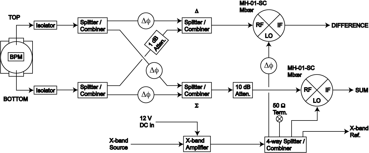
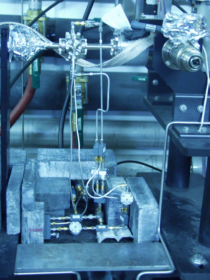
As such, the signal produced by (T &minus B) is referred to as the Difference signal and (T + B) as the Sum signal. The usual processing method, in the NLCTA striplines for example, is to extract the raw signals from each pickoff, then process the signal offline with some sort of dedicated microprocessor. However, this method of signal extraction is of no use to an experiment that requires an immediate signal response from the BPM: a signal must be extracted from the BPM on nanosecond timescales in order to provide a position measurement rapidly enough to make a number of corrections to the beam position. As such, a new processor was assembled to enable a rapid signal to be extracted from the BPM. The block diagram for the BPM processor is shown in Fig. 4.28; a photograph of the actual setup around the BPM is shown in Fig. 4.29.
| Figure 4.28: Block diagram showing the components for the FONT BPM processor. The components marked ‘Δφ’ are phase shifters. |
| Figure 4.29: The FONT BPM processor. The 4-way splitter carrying the X-band reference signal can be seen in the bottom left of the picture; the top connector carries the reference signal for the sum signal, with the third used for the difference signal and the second used to pass the signal out to the DAQ system outside the tunnel. Semi-rigid cabling is used between the isolators, connected directly to the BPM pickoffs, and the first set of splitters; conformal cable is used between the splitters in the difference path. |
The processor is a variation of the Δ/Σ method as mentioned above. In order to produce each of these signals, the signal from each of the pickoffs is split by a 2-way stripline splitter/combiner39, with one half of the signal used for the sum signal and the other half used for the difference signal. The sum signal was produced by adding the two raw pickoff signals in phase with one another, through another splitter/combiner, and mixing the resulting signal down to DC. This produces a signal whose magnitude is no longer dependent upon position, but only the charge of the passing bunch. Before allowing this signal into the mixer, a 10 dB attenuator is used to prevent this sum signal from overdriving the mixer input and causing a nonlinear signal response or damage to the mixer40. Two phase shifters41 were used in the sum signal path of both pickoffs to ensure that there was no phase difference between the two signals and that the signal attenuation was the same for both signals; the full phase setting procedure is described in Section 4.6.2.
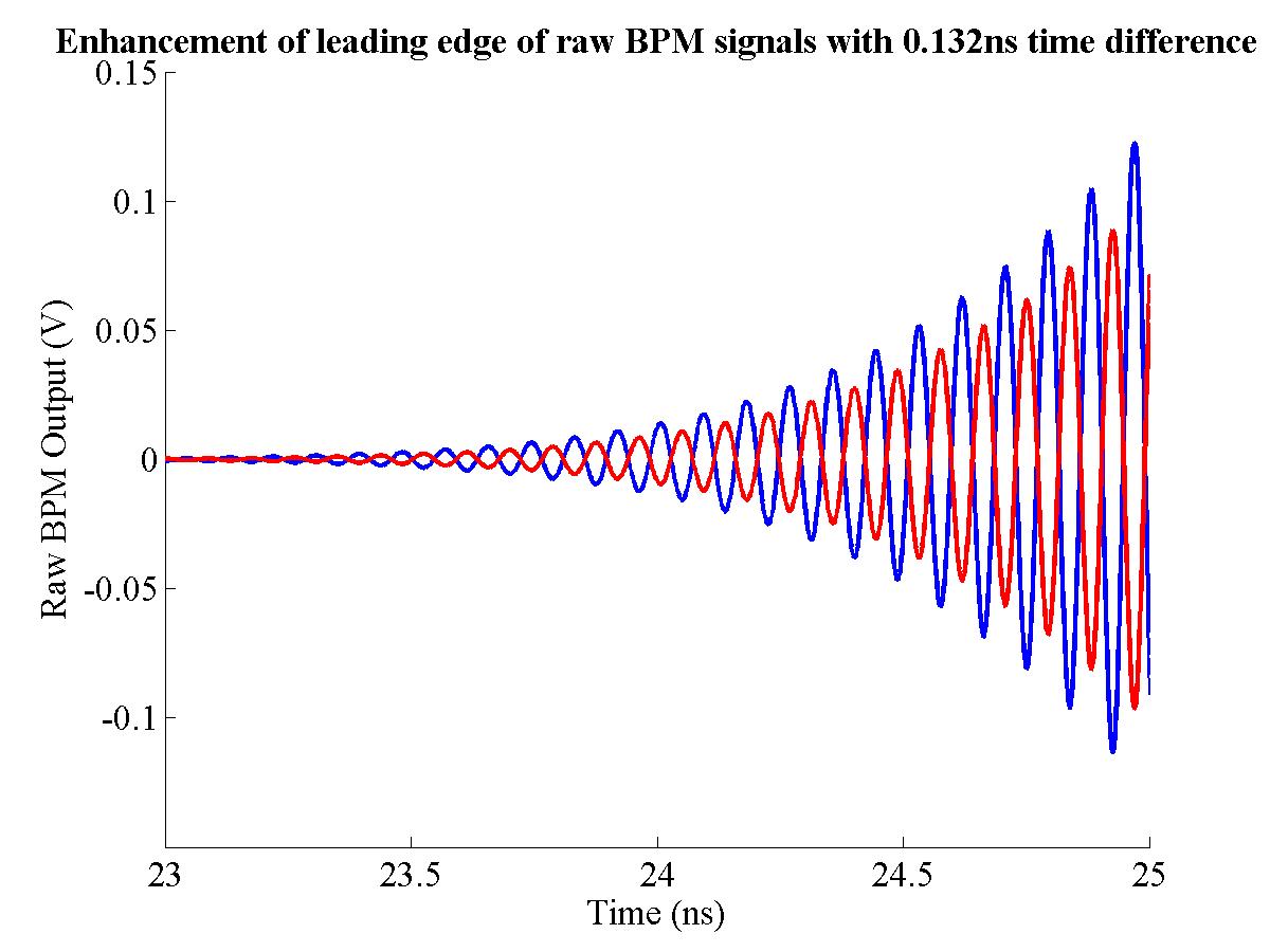
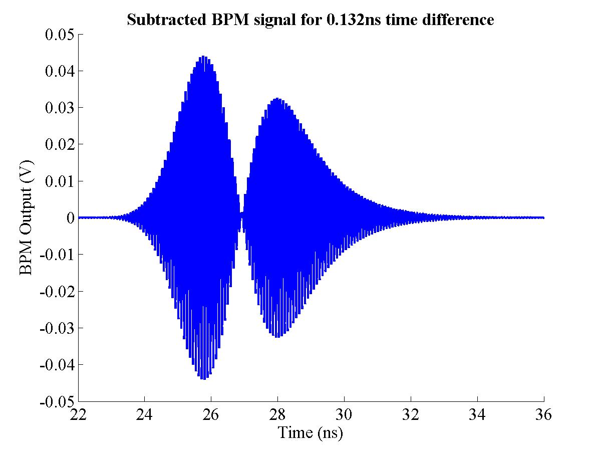
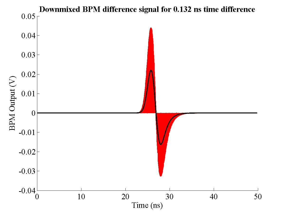
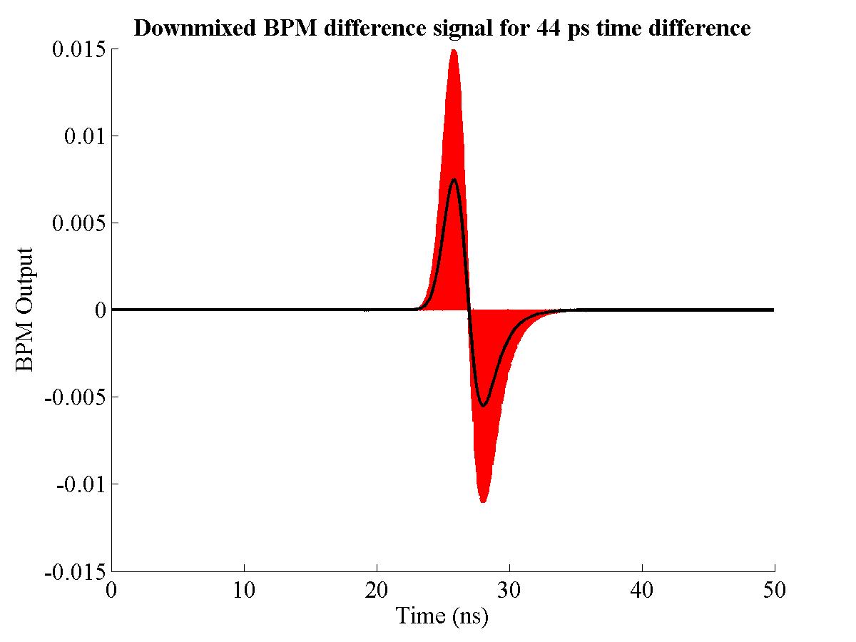
Since the signal processing had to be carried out at both high frequency (11.424 GHz) and high speed (O(5 ns)), it was deemed more advantageous to subtract the two pickoffs before downmixing to provide the required difference signal. The BPM processor takes advantage of the fact that subtracting two in-phase CW signals is the same as adding two out-of-phase signals. In order to subtract the two signals at X-band, a 180° relative phase shift is introduced into the signal path of the top pickoff via another phase shifter. In other words, before combining the signals from the pair of pickoffs to produce the difference signal, the top pickoff signal is delayed by exactly half a cycle of X-band: this is 44 ps. The two out of phase pickoff signals are now added in the same way as the sum signal, through a splitter/combiner. It is apparent that the two signals now being subtracted are no longer identical for a perfectly centred beam, due to the introduction of the 44 ps delay. However, it was expected that such a small time delay between the two pickoff signals (two orders of magnitude smaller than the time response of the BPM; see Section 4.5.2) would produce a negligible difference in signal magnitude and produce an accurate difference signal. In order that both of the pickoff signals used to produce the difference signal were of the same magnitude, a 1 dB attenuator was used in the signal path of the bottom pickoff, at the same relative location as the phase shifter, to match the signal attenuation of the phase shifter. No attenuator is needed before the input to the difference mixer as the subtraction produces a significantly smaller signal than the addition used in the sum path.
A number of improvements were made with the full two pickoff processor over the single pickoff version (Section 4.4), as discussed above. Isolators42 were introduced into the signal path, connected directly to the SMA output connector of each pickoff. This prevents any reflected signal from any of the components in the signal path from reflecting back into the BPM. The cabling between the isolators and first set of splitters was also shortened and replaced with faster semi-rigid SMA cabling. In addition, the cable lengths between components were made as short as possible — usually the length of a single male-to-male SMA connector required to connect one RF component to the next — with only the difference path making use of two short lengths of conformal cable (see Fig. 4.29). Finally, the Gunn diode was replaced with a dedicated X-band amplifier.
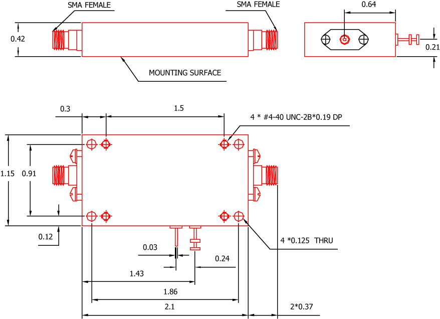
| Figure 4.30: Schematic diagram of the X-band amplifier, showing the external dimensions; dimensions are in inches [104]. |
| ||||||||||||||
|
| ||||||||||||
|
In order to provide a stable X-band reference signal for the BPM, the Gunn diode arrangement (as described in Section 4.4.3) was replaced with a dedicated X-band amplifier. The amplifier used for FONT was produced by Transcom Inc. of Taiwan; the specifications for the amplifier are shown in Table 4.5, with the external dimensions shown in Fig. 4.30. The amplifier requires a 12 V, 1.5 A DC voltage supply: this was provided by a DC power supply unit located outside the tunnel and carried into the tunnel via BNC cable. The same X-band reference signal used as the source signal for the Gunn diode was used for the amplifier, carried into the tunnel from the NLCTA RF system via 3/8-in. heliax cable. Before installation, the gain of the amplifier was briefly measured with a known input power, at 11.424 GHz, supplied by a Gigatronics Model 7100 Synthesised Signal Generator: the results are shown in Table 4.6. It is clear from this brief test that the output power tops out at just over 31 dBm, corresponding to a maximum output power of 1.35 W; it should be noted that this exceeds the maximum power output of the Gunn diode (cf. Section 4.4.3). For a supply voltage of 12.003 V, the amplifier drew a measured current of 1.31 A. Also measured were the phase and frequency stability of the amplifier output signal: no measurable deviation from the specified operating parameters was observed.
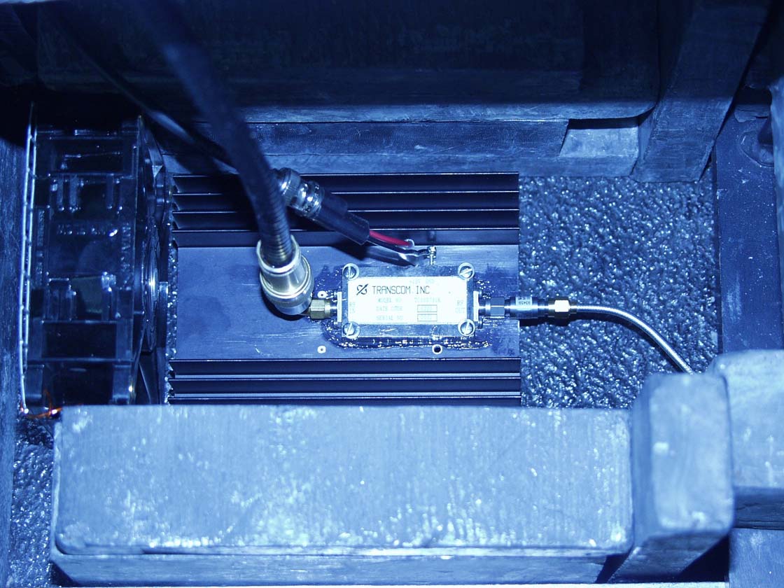
| Figure 4.31: The X-band amplifier: the RF input is on the left, with the X-band reference signal brought in on 3/8-in. heliax. The output is on the right: a 2 dB attenuator is used to drop the signal to the correct level. Power is supplied via the two pins at the top of the amplifier. The fan on the left is used to cool the enclosure; the amplifier is mounted to a black heat sink to prevent it overheating. |
The amplifier was installed underneath the beampipe in the NLCTA tunnel in place of the Gunn diode. Before installation it was mounted to a large metal heat sink, since the large quantity of heat generated by the amplifier during operation caused it to overheat and the power output and gain to drop significantly. The underside of the amplifier was first covered with a silicon gel, to provide a good thermal contact, then firmly bolted to the heat sink with four bolts. Once installed in the tunnel, the amplifier assembly was protected with lead shielding to prevent radiation damage. A 12 cm fan was placed within the shielding to encourage air flow and provide further cooling for the amplifier; small gaps were left at various points in the shielding to aid air circulation. The full amplifier assembly is shown installed in the NLCTA tunnel with some of its lead shielding in Fig. 4.31. As before, the output signal from the amplifier was split using a 4-way splitter/combiner43; this was connected to the amplifier via a 30 cm length of conformal SMA cable and an attenuator. The attenuator was used to set the reference signal for the mixers to the correct power and was set at 2 dB. Using one of the unused outputs of the 4-way splitter, the power output of the amplifier (and therefore the LO input power to the BPM processor mixers) was measured to be 17.44 dBm, compared to a required input power of 17 dBm. After 24 hours continuous running the power output had dropped to 16.87 dBm; this level remained unchanged after a further 24 hours. The fourth output of the 4-way splitter was connected to a power meter outside the tunnel via 3/8 in. heliax cable, and was used to monitor the output power of the amplifier at various intervals during data taking.
In order to provide the correctly phased signals for addition and subtraction within the BPM processor, correct setting of each of the phase shifters (see Fig. 4.28) was essential. The processor contains 4 phase shifters in total: two are used to match the phase of the sum signal44, a third sets one path of the difference signal out of phase by 180° with respect to the other, and the fourth matches the relative phase of the LO input for the two mixers. A fifth phase shifter was used to correctly set the phase of the X-band reference signal once beam running had started. A procedure for correctly setting the phase of each section of the processor was put forward by Josef Frisch and followed on each occasion that a) a component in the processor was changed or b) after a period of inactivity, usually greater than a week.
Since it would not be possible to run the beam while making the processor phase adjustments, another source of X-band signal had to be used. The best solution found was to drive each of the horizontal pickoffs with an X-band source and use the coupling between pickoffs (as shown in Fig. 4.9) to drive the vertical pickoffs. For this X-band source, the fourth output of the 4-way splitter from the X-band amplifier was used to drive the right pickoff via another phase shifter. The two phase shifters in the sum path were adjusted to both be approximately in the centre of their range; the signal path for the top pickoff was then disconnected after the isolator and the free ends terminated with 50 Ω terminators. The unused left pickoff was monitored with an Agilent E4417A Power Meter to measure the power output of the X-band source. The X-band source phase shifter was then adjusted until the output of the sum mixer reached a maximum: this indicated that the signal passing into the BPM and through the connected portion of the processor, via the bottom BPM pickoff, was in phase with the X-band reference signal when it reached the mixer45. The output of the sum mixer was measured at 18 mV, with a power output at the left pickoff of 0.80 dBm.
The bottom pickoff was then disconnected after the isolator, with the free ends terminated, and the top pickoff reconnected. The phase shifter in the top pickoff path of the sum signal was then adjusted until the sum mixer output reached a maximum of 18.5 mV. Finally, the bottom pickoff was reconnected and the output of the sum mixer measured at 37 mV; the two sum phase shifters in the sum path were then adjusted slightly to confirm that the signal output of the sum mixer was at a maximum, before being returned to their optimum positions. The whole procedure was then repeated, this time driving the left rather than the right pickoff with the X-band source signal and monitoring the power output of the right pickoff. There was no measurable difference between these results and those obtained by driving the right pickoff, indicating that the phase setting for the sum signal was likely to be sound; the power output of the right pickoff was measured to be 0.87 dBm. It should also be noted that a −2 mV offset was measured on the output of the mixer: this is present whenever a signal is input into the mixer LO port, of suitable amplitude (i.e. 17 dBm for the
Having correctly phased the two signal inputs for the sum signal, it was then necessary to adjust the difference signal. The X-band source remained driving the left pickoff, with the X-band source phase shifter left unchanged after the sum measurements in order that a consistent phase reference was present. With the top pickoff disconnected at the isolator (and the free ends terminated) and the bottom pickoff connected, the phase shifter on the LO input to the difference mixer was adjusted to make the signal produced by the difference mixer maximally negative46. With a power output of 0.93 dBm measured at the right pickoff, the difference mixer output reached a maximally negative value of −40 mV; adjusting for the −2 mV offset of the mixer gives a value of −38 mV. The bottom pickoff was then disconnected at the isolator (with the free ends terminated) and the top pickoff reconnected. The phase shifter in the difference signal path from the top pickoff was then adjusted to maximise the output of the difference mixer at 35 mV, or 37 mV when accounting for the mixer offset. Finally, the bottom pickoff was reconnected and the output of the difference mixer measured to ensure a zero output: after setting the phase shifter from the top pickoff to its optimum position, the output of the difference mixer was measured to be
A problem exists with this phase setting procedure, however, since it is impossible to use the true source of X-band signal for these measurements: this signal source is the beam itself. Since one cannot run the beam whilst a person is in the tunnel, and one cannot adjust the BPM processor phase shifters from outside the tunnel, the only satisfactory solution was to drive one of the two unused pickoffs with an X-band signal source. It is highly unlikely that the phase of a signal produced by injecting a signal into the BPM through one of the unused pickoffs is the same as that produced by the beam itself. However, the procedure is not completely without value, since one is concerned with the relative difference between the two pickoffs. Given that there was no measurable difference in the setting of each phase shifter when the right, rather than the left pickoff was used as the X-band source, it is probable that the relative phase of each portion of the BPM processor has been set correctly. It is an open question how one could test these settings more rigorously, since one cannot inject an X-band signal into the BPM via the beampipe as the diameter of the pipe is designed not to pass X-band (see Section 4.3.1).
The final part of the phase setting procedure is to correctly set the phase of the X-band reference signal. This was to ensure that the two LO inputs to the sum and difference mixers were exactly in phase with the BPM signal produced in response to the passing beam. An X-band phase shifter was inserted into the signal path of the reference signal before it entered the tunnel to allow the phase to be set remotely. The setting of this phase required the beam to be running, but was not dependent upon the beam pulse type (see Table 3.3). Once running, the beam was steered upwards to produce a positive difference signal. Initially the phase shifter was adjusted to maximise first the sum, then the difference signal. The phase was then adjusted to find the null points (±90° from being exactly in phase, giving zero output; see footnote 45) for both the sum and difference signals.
A phase difference of approximately 20° was measured between the sum and difference output: the phase shifter was therefore set between these two values, 10° away from being exactly in phase with each signal. This 20° phase difference is an indication of the inaccuracy present in the BPM processor phase setting procedure; however, a phase difference between beam and reference of 10° was considered acceptable. For the long pulse beam, a phase slew of approximately 20° was observed along the length of the 170 ns pulse; this was later corroborated by independent measurements made by Chris Adolphsen. The BPM processor is largely insensitive to such a phase slew, as long as the reference signal is close to being exactly in phase with the beam. It was also of note that the majority of this phase slew is present at the leading and trailing edges of the pulse, with the central 100 ns of the pulse stable to ~5°. This final phase setting procedure was carried out more often than that required for the BPM processor, since the reference phase was observed to drift by up to 90° over a 24 hour period.
Although the BPM was designed to measure the full 170 ns long pulse, it was also possible to use it to measure the 2 ns short pulse beam. The advantage of using the short pulse beam is that more trustworthy corroborative evidence is available for the BPM position measurements: as noted in Section 4.2, the NLCTA stripline BPM's were only sensitive to beam pulses around a nanosecond in length. For times longer than ~1 ns, the reflections caused by the striplines (see Fig. 3.6) cancel the original impulse beam response, giving no output. However, for the first 1 ns of the beam pulse, the reflected pulse has not yet had time to arrive at the front edge of the stripline, so a position measurement can be made. It is therefore possible to measure the position of the leading edge of the long pulse beam, but a much more accurate measurement is possible for the short pulse beam.
| Figure 4.32: Blow-up of the area of the NLCTA around the FONT BPM, showing the NLCTA stripline BPM's recorded during the FONT BPM tests (adapted from [76]). The ‘1’ at the end of each BPM ID indicates that y position is being measured (a ‘0’ would indicate x position). |
Data from the NLCTA stripline BPM's is recorded using the NLCTA section of the SLAC Control Program (SCP). The SCP can record both the x and y position as measured by the BPM, plus the Total Measured Intensity (TMIT): the TMIT measurement is similar to the sum signal produced by the FONT BPM processor and is a measure of the beam charge observed by the BPM. Due to the multiplexing used in the stripline BPM data acquisition system, only one plane is recorded for each beam pulse i.e. only x or y can be recorded for any single pulse, plus the associated TMIT. As such, when using the SCP to record data, it is only possible to record beam position for one of the two axes. Two methods of data collection are available: buffered data and correlated data. Buffered data acquisition is the measurement of n consecutive pulses for identical beam conditions. Correlated data, also known as ‘correlation plotting’ is the acquisition of n consecutive pulses while incrementally changing the beam orbit; this usually involves the steering of the beam with one or two dipoles, and correlating the beam position measured at each BPM to the current/field of each dipole.
For the FONT BPM tests, only the y position of the beam was measured, since the FONT BPM was only set up to record the vertical beam position. The SCP was programmed to record the Y position and TMIT of 7 NLCTA stripline BPM's: 1451, 1551, 1651, 1761, 1811, 1871 and 1921. Each BPM is mounted inside a quadrupole magnet: the location of each of these BPM's, along with the FONT BPM, is shown in Fig. 4.32. The most important of these BPM's is 1761, since the FONT BPM is installed just upstream and there are no magnetic elements between them; it is possible therefore to use the position measurement of BPM 1761 as a comparable measurement for the beam at the FONT BPM, since there is only ~40 cm of drift space between the two. The output signals from the FONT BPM processor were brought out of the NLCTA tunnel on 3/8 in. heliax cable and connected to a Tektronix digitising oscilloscope. Using the scope's GPIB interface and a GPIB-TCP/IP interface box, the data for each pulse was extracted from the scope by a PC running Matlab, allowing the DAQ and data manipulation to be integrated into a single Matlab routine.
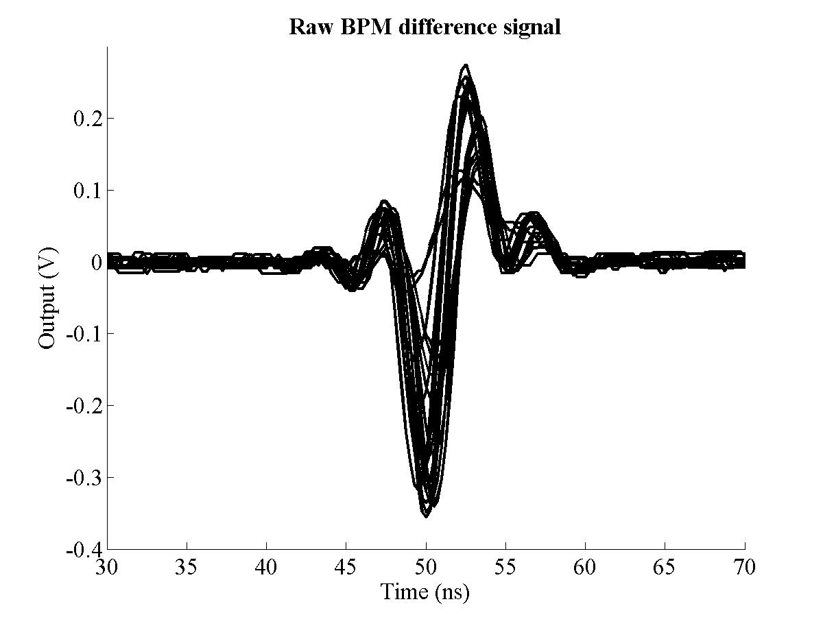
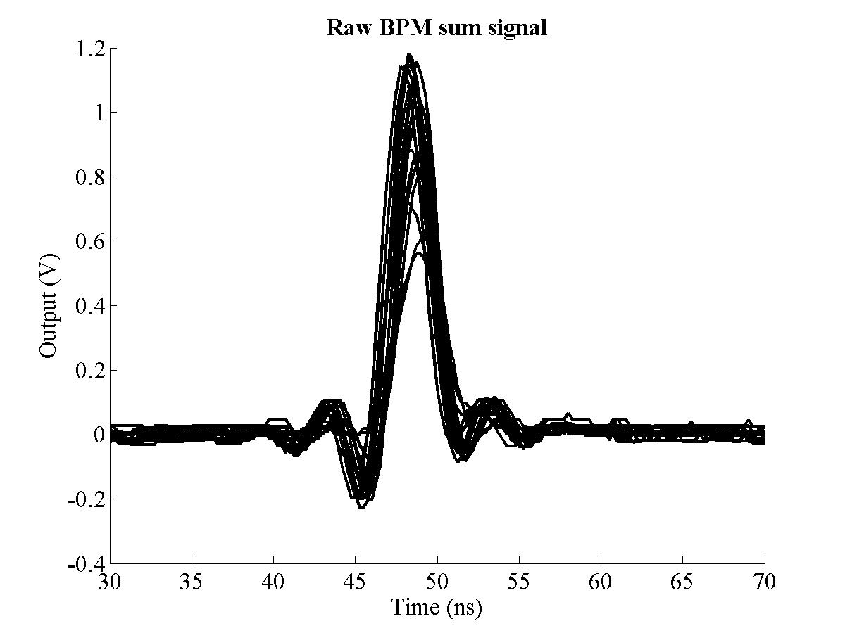
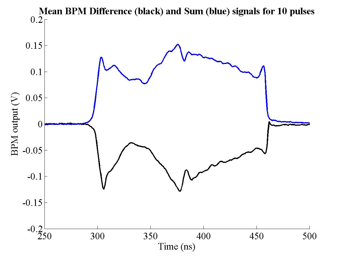
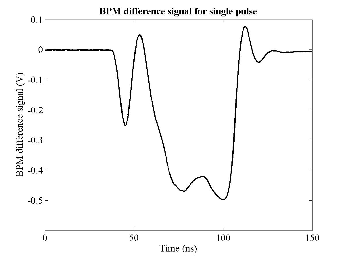
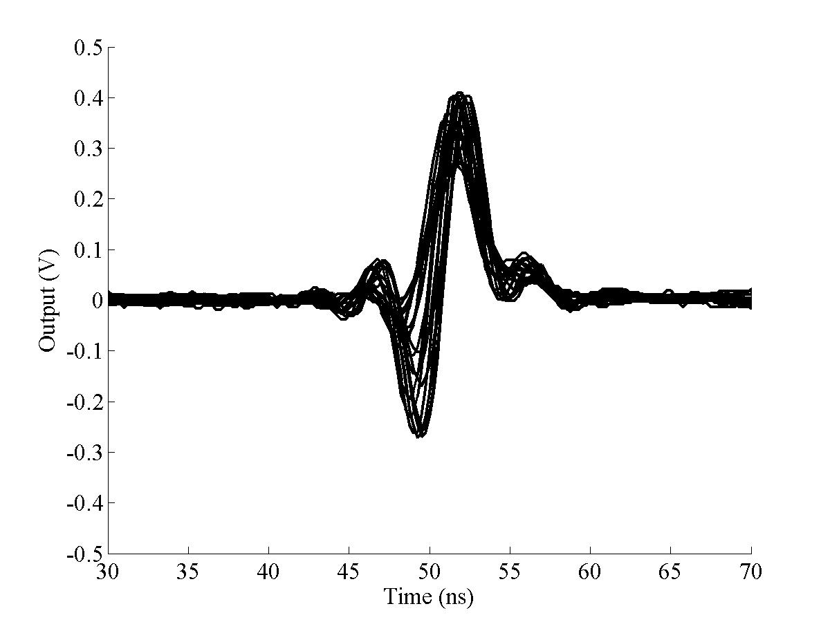
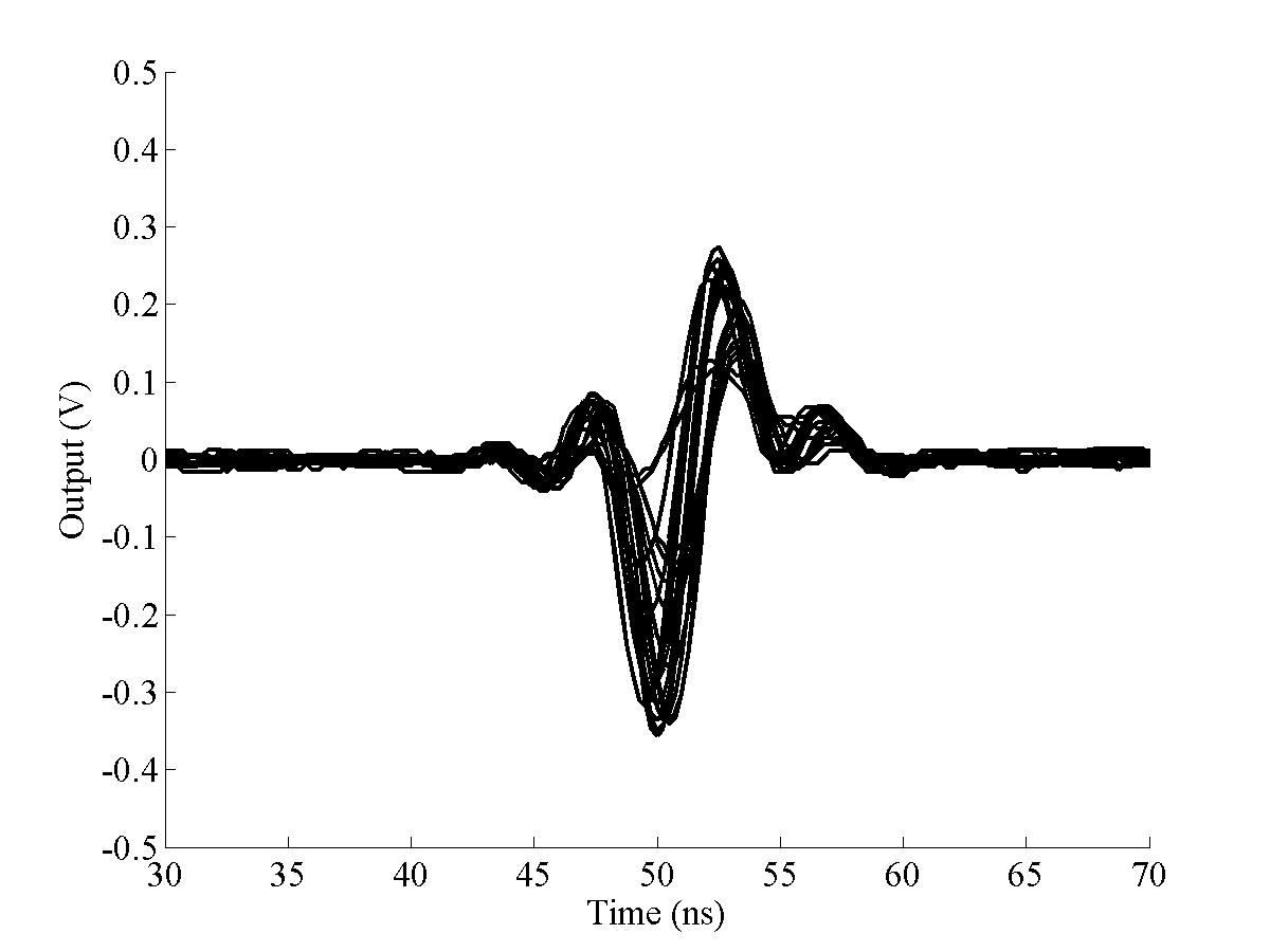
| Figure 4.33: The raw difference signal produced by the FONT BPM processor for the short pulse beam. Note the large overshoot that appears at 50 ns; plot shows 20 beam pulses. |
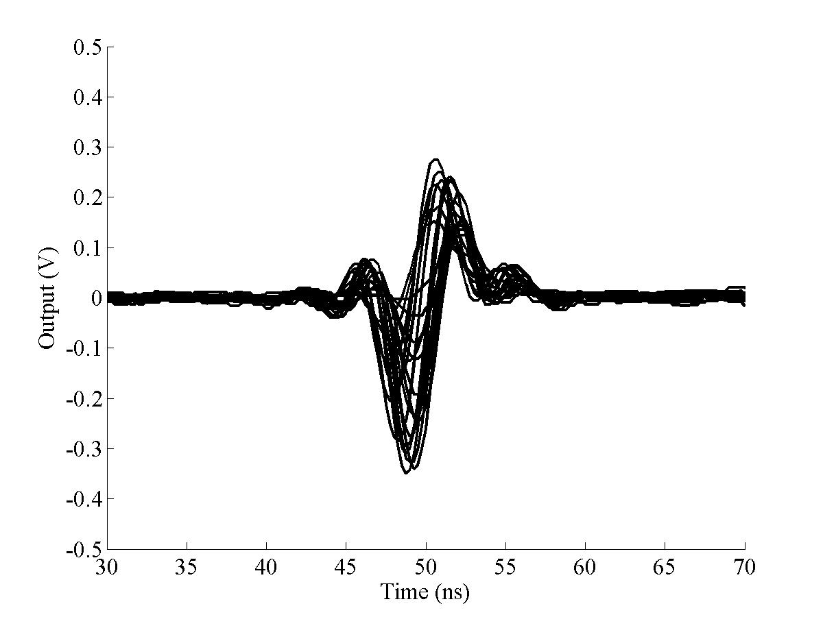
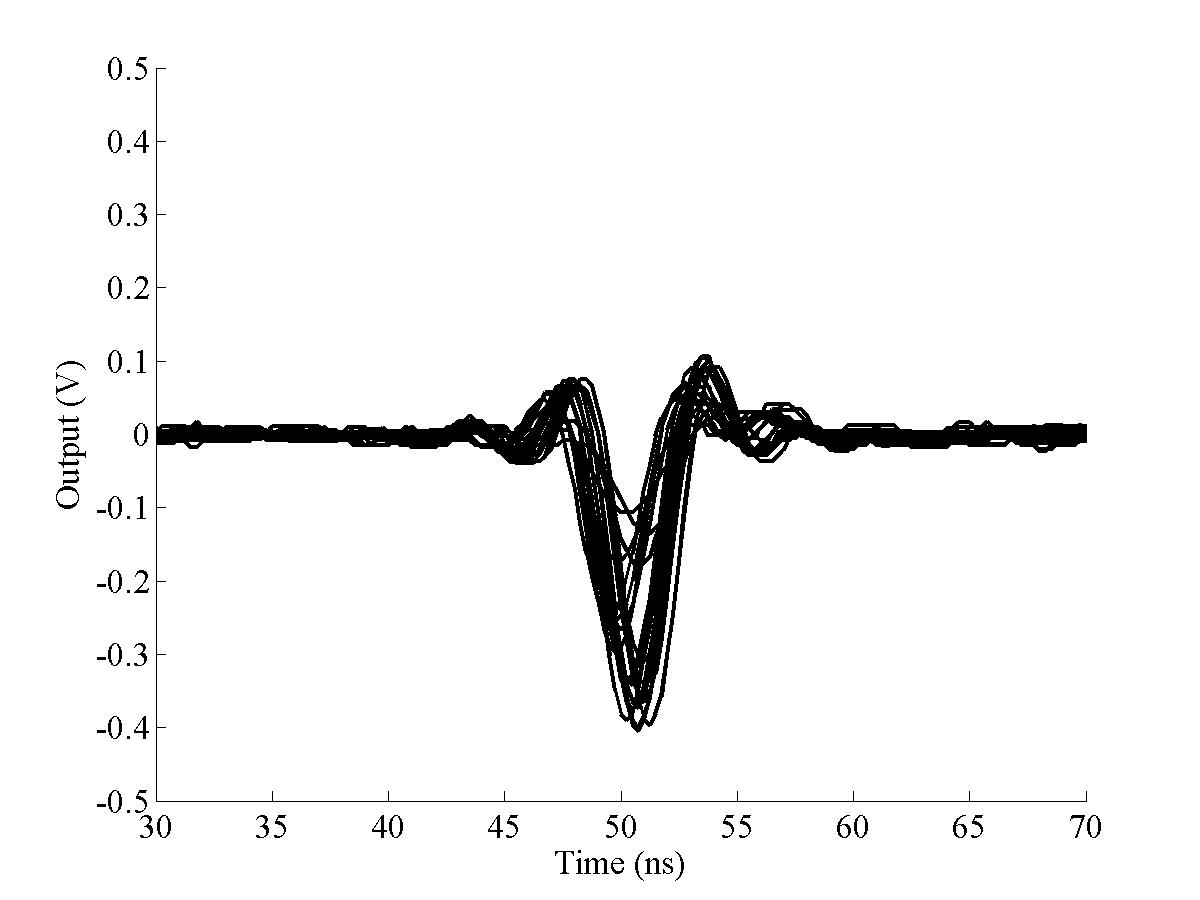
| Figure 4.34: The raw sum signal produced by the FONT BPM processor for the short pulse beam; plot shows 20 beam pulses. |
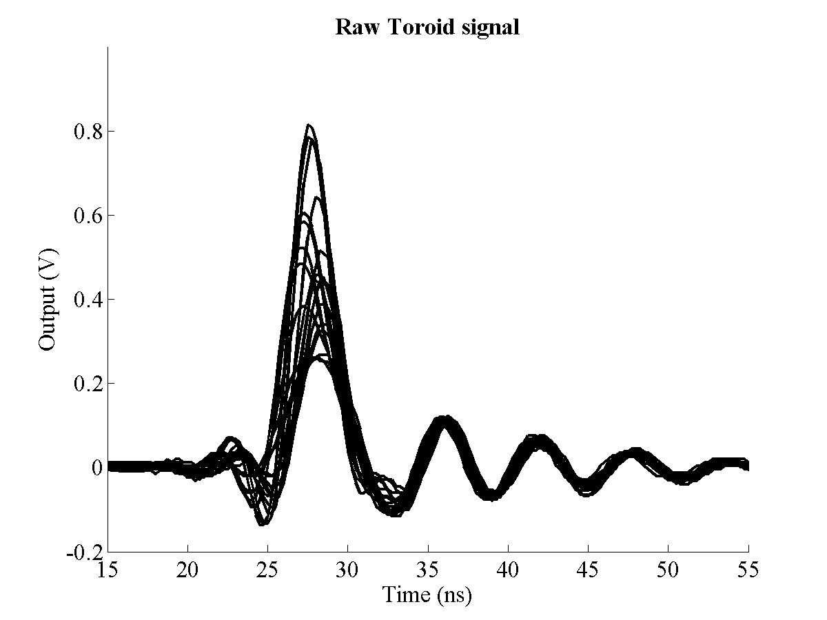
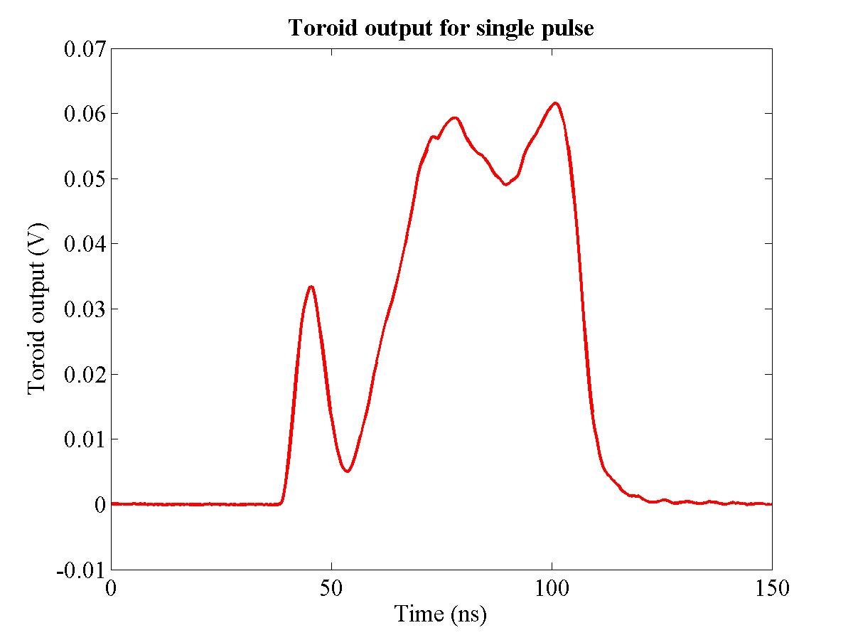
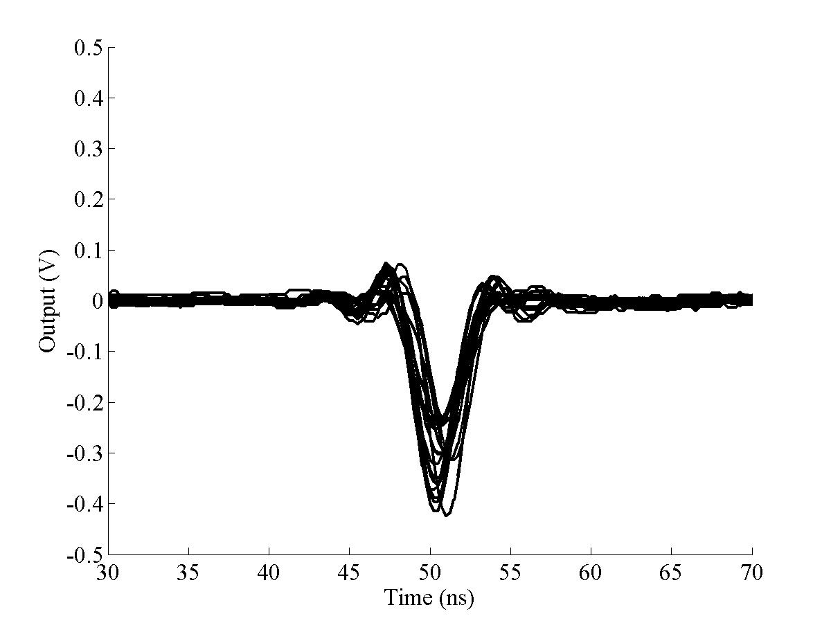
| Figure 4.35: The output of toroid 1750 for the short pulse beam; plot shows 20 beam pulses. The output (until the ringing starts at ~35 ns) is similar to that of the FONT BPM sum signal (Fig. 4.34). |
The sum and difference outputs of the FONT BPM processor in response to the short pulse beam are shown in Figs. 4.33 and 4.34; the corresponding output of Toroid 1750, situated between the FONT BPM and BPM 1761, is shown in Fig. 4.35. For these measurements, the beam was steered as close to the centre of the BPM as possible using the y corrector (YCOR 1650) of QD1650, the quadrupole upstream of the BPM. YCOR 1650 was chosen as there is only drift space between QD1650 and the FONT BPM. The first clear feature is the enormous double peak that appears on the BPM difference signal. Since the difference signal is a convolution of both beam position and charge, this would appear to indicate that the position varied wildly midway through the pulse, since the charge cannot be negative. A greater analysis of this signal overshoot is given in Section 4.7.2.
|

|
||||
| (a) 4.0 G-m | (b) 2.5 G-m | ||||
|
|
||||
| (c) 1.29 G-m | (d) 1.29 G-m | ||||
|
|
||||
| (e) −0.5 G-m | (f) −2.0 G-m | ||||
| |||||
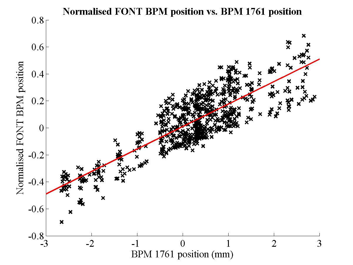
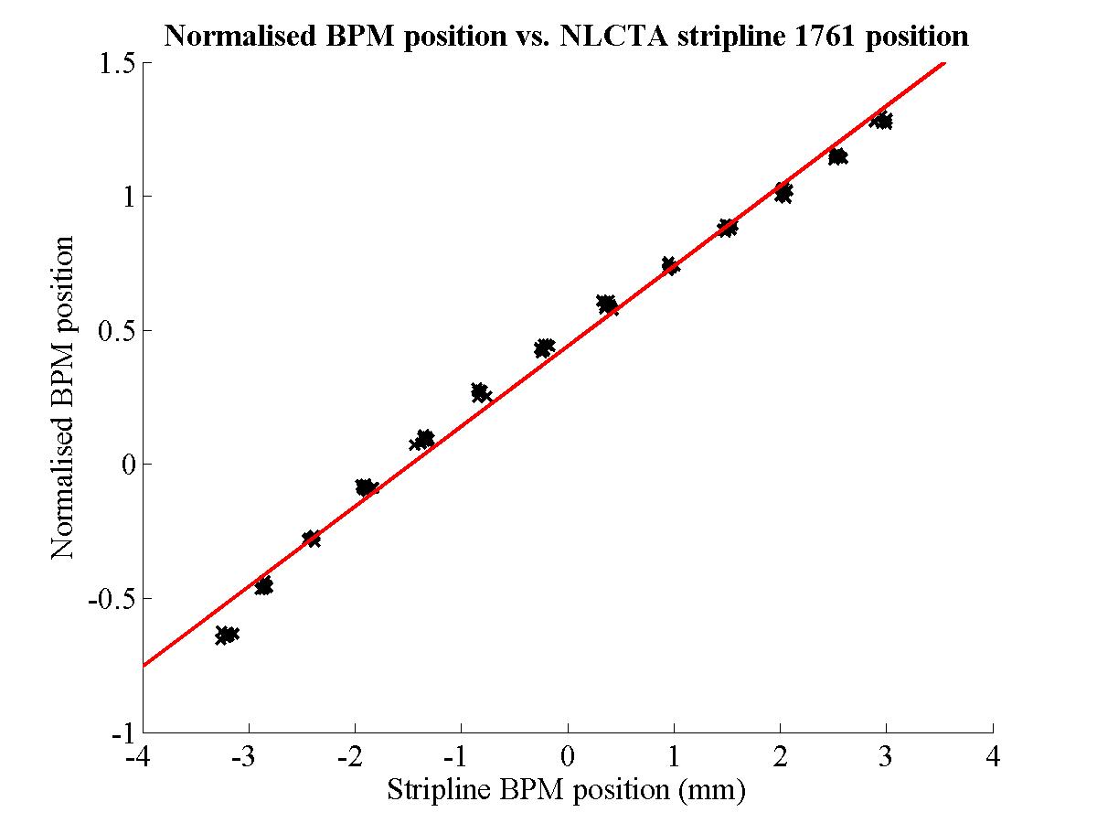
| Figure 4.37: Normalised FONT BPM position vs. BPM 1761 position for 20 beam pulses at 35 different magnet settings. Normalised position is the max − min signal divided by the mean of the corresponding sum signal. The red line is a line of best fit produced through a χ2 minimisation. |
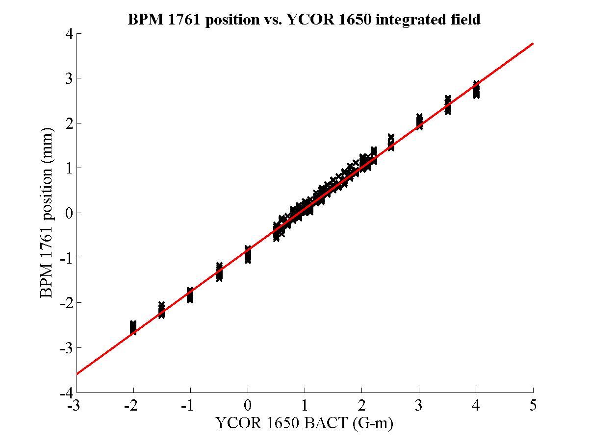
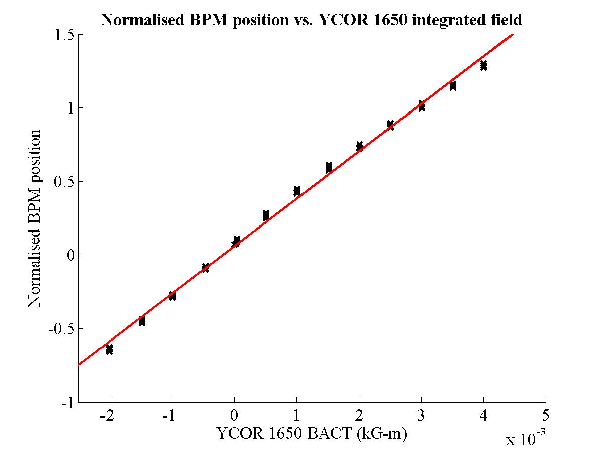
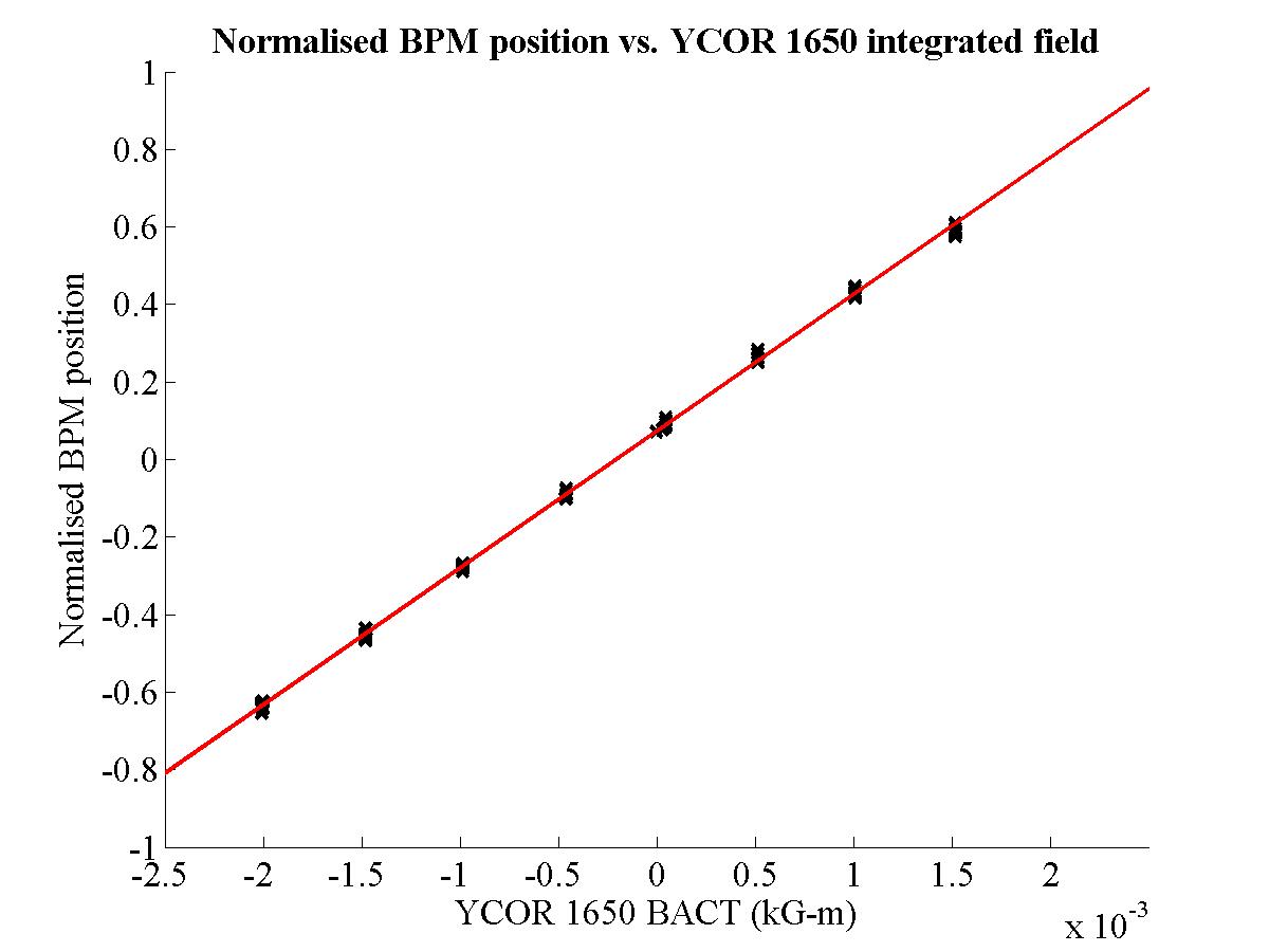
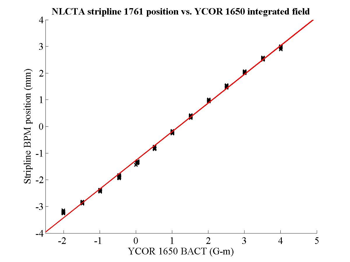
| Figure 4.38: BPM 1761 y position as a function of the integrated field, in G-m, of YCOR 1650 for 20 beam pulses at 35 different magnet settings. ‘BACT’ is the ‘actual’ integrated magnetic field, as calculated from the measured current in the magnet. The red line is a line of best fit produced through a χ2 minimisation. |
However, even though the BPM does not produce an expected position signal, it does appear to produce a response that varies with position. This can be seen in Fig. 4.36: this figure shows the variation of the BPM difference signal as a function of the integrated field, B.dL (in Gauss-metres), of YCOR 1650. An increasing field strength of YCOR 1650 corresponds to the beam being steered upwards: the beam is at its lowest at the FONT BPM for B.dL = −2.0 G-m and at its highest for B.dL = 4.0 G-m. If the BPM were performing in an ideal way, the profile for each pulse should follow the shape of the sum signal (Fig. 4.34), with a magnitude proportional to the beam position i.e. a positive peak for a beam high of centre and a negative peak for a beam low of centre. It would initially appear that, for each of the beam pulses shown in Fig. 4.33, there is no such correspondence between beam position and pulse magnitude, primarily due to the double peak that appears in the centre of most of the pulses. However, closer inspection reveals that the relative height of the two central peaks (one positive, one negative) does show an approximate dependence on the magnet field strength. By taking the difference between these two peaks (i.e. max − min), an approximate correspondence is observed between the FONT BPM signal and the measured beam position.
The y position measured by BPM 1761 is shown plotted against the normalised position for the FONT BPM in Fig. 4.37 for 20 pulses at 35 different magnet strengths: the normalised position is produced by dividing the max − min signal, for each pulse, by the mean value of the sum signal over the length of the pulse, in an approximation of the Δ/Σ method. This plot should be compared to Fig. 4.38, which shows the variation in vertical beam position, as measured by BPM 1761, as a function of the integrated field strength of YCOR 1650. Fig. 4.38 clearly shows that there is a smooth linear relationship between the variation of dipole field strength and the measured beam position downstream of that magnet: this is exactly what one would expect, given that there are no magnetic elements between YCOR 1650 and BPM 1761 (see Fig. 4.32). Due to the short pulse length, the position as measured by the stripline BPM can be taken as a good measurement of actual beam position, not only at BPM 1761 but also at the FONT BPM just upstream47. As such, Fig. 4.37 shows that, although the FONT BPM performs considerably less well than the stripline, it does respond to some degree to the actual position of the beam. Although the large spread in the normalised position of the FONT BPM is a significant fraction of the full measured range — 0.4 normalised units spread for a full range of 1.4 normalised units — there is still a clear trend that follows the line of best fit.
| Figure 4.39: The sum signal of the X-band BPM as a function of the toroid output for 700 pulses with the short pulse beam. Both signals are calculated using the peak value of each pulse. |
Fig. 4.37 also shows that the electrical centres of the FONT BPM and BPM 1761 are closely matched, since the fitted line passes very close to (0,0). However, it is also apparent when comparing Fig. 4.37 to Fig. 4.38 that the signal noise that appears on the normalised X-band BPM signal is not a result of actual jitter on the beam, since the position as measured by BPM 1761 shows an r.m.s. vertical beam jitter of ~70 µm: this is much less than the full range of 5 mm. The jitter on the X-band BPM normalised position measurement is some 20 times larger than that of the stripline BPM and is therefore likely to be a result of poor measurement by the X-band BPM, rather than true beam jitter. Another example of the poor short pulse performance of the FONT BPM is shown in Fig. 4.39. The peak output of the FONT BPM sum signal is plotted against the peak output of the toroid for each pulse. Given that both of these methods should give accurate measurements of the bunch charge of the beam, the distribution that appears in Fig. 4.39 is alarming: the expected positive linear relationship between two devices measuring the same quantity is clearly absent. No satisfactory explanation for this behaviour has yet been put forward. It is clear, however, that the X-band BPM behaves poorly in response to the short pulse beam.
As mentioned in the previous section, the double peak (henceforth referred to as “overshoot”) that appears on the BPM difference signal (Fig. 4.33) was unexpected: due to the sharpness of this peak and the relative variation of the sizes of the positive and negative peaks with beam position, as shown in Fig. 4.36, it is unlikely that this peak is a feature of the beam itself. The likelihood is that this overshoot is due to the BPM processor, with the following possible explanations:
A third possible option was that the phase slew across the pulse was causing the overshoot. As observed with the phase setting procedure, there is approximately a 20° phase slew over the length of the pulse. If the centre of such a signal was 90° out of phase with the reference signal, then the result of mixing two such signals together would produce a signal with zero output at this 90° point. The sign of the signal would then be positive before and negative after this 90° point if the reference signal was 90° ahead of the beam signal; the opposite would be true if the reference signal was 90° behind. However, the phase difference between reference and difference signals was only about 10° (see Section 4.6.2). Therefore, such an effect would not be noticeable, since the phase difference between the difference and X-band reference signals was set to be no more than 20°.
| Figure 4.40: RC-filtered Gaussian pulse used to simulate bunch train for short pulse beam. |
| Figure 4.41: Two RC-filtered Gaussian pulses, used to simulate the short pulse response for the top and bottom pickoffs with a 132 ps delay between pickoff signals. The top pickoff is shown in blue, with the delayed bottom pickoff shown in red. |
In an attempt to diagnose the cause of the problem from the two remaining possibilities, the various BPM signals input to and produced by the BPM processor were simulated in Matlab. The first task was to correctly simulate the pulse output by the BPM in response to the short pulse beam. In order to produce this beam pulse, the RC-filtered Gaussian pulse that was previously generated as part of the characterisation of the BPM response was used (see Section 4.5.2). The fitted parameters shown in Fig. 4.24 were used to produce the simulated pulse of Fig. 4.40. This pulse shape — simulating a Gaussian distribution of charge along the length of the bunch train — was considered to be a better approximation than that produced by the RC-filtered square pulse when compared to the real BPM sum signal data shown in Fig. 4.34. The Gaussian pulse shape was then used to modulate an 11.424 GHz signal to produce a facsimile of the real X-band output of each pickoff in response to the beam.
| Figure 4.42: X-band signal modulated with two RC-filtered Gaussian pulses, used to simulate the short pulse response for the top and bottom pickoffs with a 132 ps delay between pickoff signals. The top pickoff is shown in blue, with the delayed bottom pickoff shown in red. |
| Figure 4.43: The leading edges of the signals shown in Fig. 4.42: note the magnitude difference between the two pulses corresponding to the 132 ps delay. The top pickoff is shown in blue, with the delayed bottom pickoff shown in red. |
| Figure 4.44: The simulated X-band signal produced by adding the two pulses shown in Fig. 4.42: the phase of this signal contains the information on whether the resulting downmixed pulse will be positive or negative. |
The initial hypothesis was that an extra delay of 88 ps — one cycle of X-band — was causing the overshoot seen in the BPM difference signal. Two identical pulses were therefore created, as described above, in order to simulate the signal produced by the top and bottom pickoffs in response to the short pulse beam. They were then used to modulate an X-band signal to produce the true X-band output of each pickoff. The signal representing the bottom pickoff was then delayed by 132 ps with respect to the top signal: this is a delay of 1-1/2 cycles of X-band, corresponding to a 180° phase delay plus an extra cycle of delay introduced erroneously. The simulated pulse envelopes are shown in Fig. 4.41, with the resulting X-band signals shown in Fig. 4.42. An enhancement of the first 2 ns of Fig. 4.42 is shown in Fig. 4.43: note that the blue trace corresponding to the top pickoff signal can be seen to rise earlier than the red trace (bottom pickoff) as a result of the 132 ps delay in the bottom pickoff signal introduced into the simulation. The next stage in the processor is to subtract these two signals produced by the BPM pickoffs: this is achieved by adding the two signals, through a splitter/combiner (see Section 4.6 and Fig. 4.28), and produces the signal shown in Fig. 4.44.
| Figure 4.45: The simulated downmixed X-band signal produced by mixing the pulse shown in Fig. 4.44 with an X-band reference signal and low pass filtering the resulting output. The DC component, output by the mixer, is shown overlaid in black: this is the difference signal output by the FONT BPM processor. Note the similarity to the measured difference signal shown in Fig. 4.33. |
After subtracting the two raw pickoff signals to produce a difference signal at X-band, the final processor stage is to mix this difference signal at 11.424 GHz and low-pass filter it to recover the DC component. The mixed signal is produced by multiplying the difference signal with a reference signal at 11.424 GHz: the phase of this reference signal is crucial, since it must be exactly in phase with the original beam pulse. In terms of the simulation, this means that the reference signal is exactly in phase with the modulated X-band signal used for the top pickoff. The resulting signal is a convolution of the sum and difference frequencies (see Eq. (3.11)): as before, the DC difference frequency is the signal of interest; the 22.848 GHz sum frequency is removed by low pass filtering. The low pass filter used for the simulations was a 4-pole Bessel filter with fc = 200 MHz, as is used for the real BPM processor. The downmixed signal is shown in Fig. 4.45: the mixed signal is shown in red, with the filtered DC component shown in black. Note that this signal is surprisingly similar to the true FONT BPM difference signal shown in Fig. 4.33, but with the peaks reversed. The reason for this peak reversal is that, in the simulation, the signal from the bottom pickoff arrives later than that from the top pickoff; in the real processor it is the other way round (see Fig. 4.28).
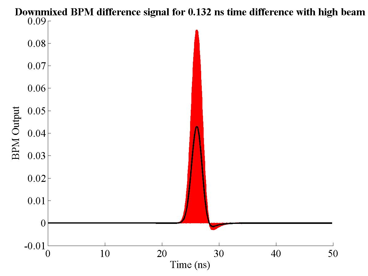
|
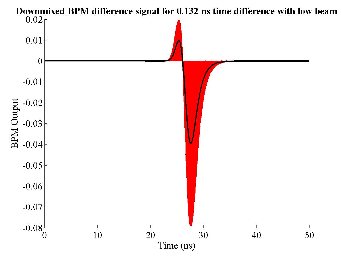
|
||||
| (a) High beam | (b) Low beam | ||||
|
|||||
In addition to the centred beam, both a high and low beam were simulated by increasing the magnitude of one of the signals shown in Fig. 4.41 with respect to the other by 10%. No attempt was made to ascertain the actual signal ratios for a particular beam position; it was not anticipated, however, that this would cause any problems with the realism of the simulation48. The simulated response for an off-centre beam is shown in Fig. 4.46: again, note the similarity between these simulations and the actual difference signal shown in Fig. 4.36. Although in each case one of the two peaks shrinks noticeably — the positive peak for a low beam and the negative peak for the high beam — it is still present in each case. This ‘peak shrinking’ can also be seen in the real difference signal for the various beam positions shown in Fig. 4.36.
| Figure 4.47: The simulated downmixed X-band signal produced for the ideal time delay between pickoffs of 44 ps; the DC component, output by the mixer, is shown overlaid in black. Note the similarity to the measured difference signal shown in Fig. 4.33. |
Having simulated the beam for an 88 ps error in the relative signal paths of the two pickoffs, the next step is to compare this result to the X-band BPM output for the correct signal delays. The simulation proceeds in the same way as described above, but with a relative delay between the two pickoffs of 44 ps rather than 132 ps. This 44 ps delay is used to turn the addition of the two signals into a subtraction at X-band, as described previously. The simulated downmixed difference signal for a 44 ps signal delay is shown in Fig. 4.47. Note that the signal shape in Fig. 4.47 is almost identical to that shown in Fig. 4.45. The only obvious difference between the two figures is the magnitude of each of the two peaks in both figures, which are noticeably larger for the longer time delay shown in Fig. 4.45: the output signal, shown in black, for the 44 ps delay of Fig. 4.47 is around 7.5 mV, about a third of the magnitude of the same signal in Fig. 4.45 at 22 mV. This point is crucial: the implication is that, for a perfectly functioning X-band BPM, the electronics will still produce the double peaked signal seen in Fig. 4.33. Even as small a difference in signal path as 44 ps makes the difference between an exact cancellation with a centred beam and the large peaks resulting from an inexact cancellation that appear in the real signals. This surprising result is due to the nature of the difference-over-sum procedure, where one takes a very small difference of very large signals: the very small time difference produces the same small signal difference, but due to the large raw signals produced by each pickoff this inexact cancellation produces the enormous double peaks seen in Fig. 4.33. The implication is that this will also be true for the long pulse beam: a description of the simulation as applied to the long pulse beam is given in Section 4.8.3.
| Figure 4.48: The simulated downmixed X-band signal produced for a relative phase error between pickoff signals of 10°. The DC component is shown overlaid in black: note that it is essentially zero for the entire pulse. |
In addition to the signal path difference, a phase error was also introduced to the simulation to test the effect of a phase difference between the two signal paths of the top and bottom pickoffs, resulting from an incorrect setting on one of the phase shifters. The simulation was identical to that previously described, but with a 10° phase difference introduced between the two signals corresponding to the two pickoffs, rather than a 44 ps time difference (a 10° phase error between the reference and difference signals was measured in Section 4.6.2). The simulation was therefore slightly artificial in the sense that any time delay between the pickoffs, necessary in the real system to enable signal cancellation by addition, was removed to try and isolate the effect of the phase difference. The result of this simulation is shown in Fig. 4.48: again, the mixed signal is shown in red, with the downmixed DC component shown in black. It is clear to see that the DC component is essentially zero, demonstrating that the cause of the BPM overshoot is not a result of the phase difference between pickoffs.
The conclusion is that the true cause of the BPM overshoot, or double peak, is the necessary 44 ps delay introduced into the processor to enable signal cancellation at X-band. It is therefore possible to refute the initial claim that this time difference would make no difference to the resulting downmixed signal (see above). Given the timescales involved, and comparing this time delay to the fitted time constant of the BPM of 1.5 ns (see Section 4.5.2), it is indeed surprising that such a small time delay should make a difference. It is an interesting question as to the point at which a relative time delay in the raw BPM pickoff signals no longer becomes important: clearly, on the basis of these simulations, the delay must be substantially more than two orders of magnitude smaller than the time response of the BPM pickoff before it becomes negligible.
Although the attempts to measure the position of the short pulse beam, as detailed in the previous section, were largely unsuccessful, a true test of the performance of the FONT BPM would be in response to the long pulse beam. The maximum pulse length available at the NLCTA is on the order of 180 ns, being the maximum portion of the X-band pulse used to drive the structures that is capable of stable beam acceleration. The maximum usable pulse length is on the order of 170 ns; the pulse length of the gun itself is around 220 ns. Although a much better response was expected from the FONT BPM in response to the long pulse beam, the associated disadvantage was that the position measurement of the NLCTA striplines would be much less reliable. Since the rise time of the long pulse beam is much longer than that of the short pulse beam, only those pulses which rise particularly quickly will register with the striplines, for reasons explained in Section 4.7. However, the advantage of the long pulse beam is that a much more reliable output is obtained from the toroid. For the short pulse, the ringing that appears at the end of the pulse (see Fig. 4.35) dominates; for the longer timescales associated with the 170 ns beam such ringing should be of minor significance.
| Figure 4.49: The raw output of the BPM processor sum signal (blue) and toroid output (red) for the long pulse beam; beam pulse is approximately 160 ns long. |
| Figure 4.50: The BPM processor sum signal (blue) and toroid output (red) for the long pulse beam. The toroid signal is scaled up by a factor of five to show the close profile match with the sum signal. Data is the same as that shown in Fig. 4.49. |
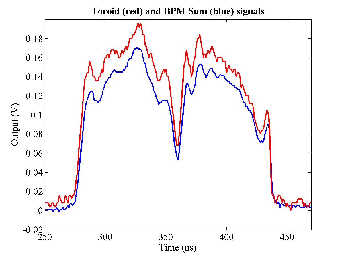
|
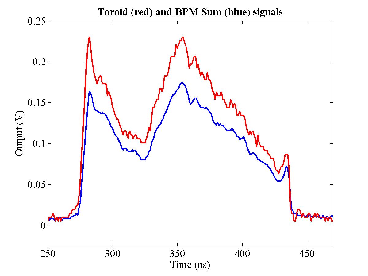
|
||||
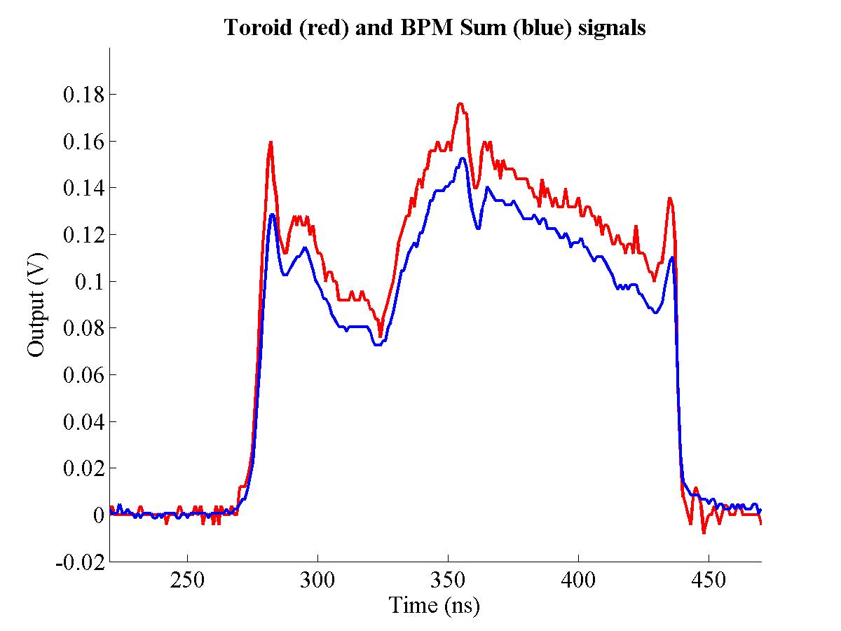
|
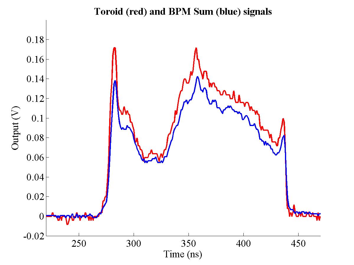
|
||||
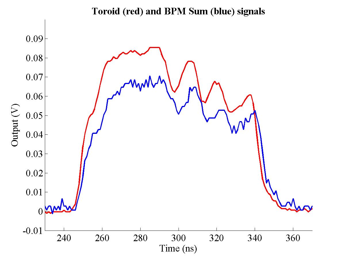
|
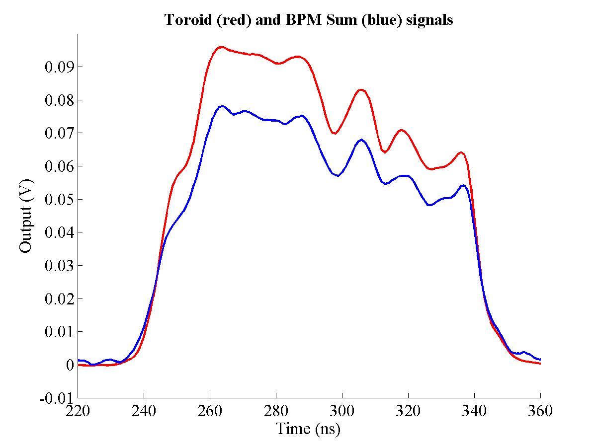
|
||||
| |||||
As described previously, the BPM processor sum signal should be an accurate representation of the beam charge. The long pulse response of the sum signal, along with the toroid, is shown in Fig. 4.49. The output of the BPM processor sum signal, shown in blue, is considerably larger than the toroid: this is due to the enhanced beam coupling of the X-band BPM to the beam as a result of its resonant behaviour. A modified version of this figure is shown Fig. 4.50, in which the toroid signal is scaled by a factor of five to match the magnitude of the BPM sum signal. The toroid is considered to be an accurate measure of the beam charge for the whole train: note that the two curves follow one another very closely. All of the features that appear on the toroid signal are clearly replicated on the sum signal. Another demonstration of the close match of these two beam charge measurement methods can be seen in Fig. 4.51. 6 different pulses are shown, each taken on different occasions: note the difference in pulse shape between each of the plots. It is clear on this evidence that the BPM sum signal is, as mentioned previously, as good a measure of the beam charge as the toroid.
This charge comparison can be taken a stage further by looking at the total charge measured for each pulse through both methods. By taking the mean signal value for each pulse, it is possible to compare the total charge measured through each method: this is shown in Fig. 4.52. In this figure, the mean BPM sum signal is plotted against the mean toroid signal for each of 130 consecutive pulses. The average signal value is taken between 210 and 370 ns (see Fig. 4.49): the limits are chosen to be wider than the pulse to ensure that the signal has settled sufficiently. Since the two methods are measuring the same quantity, one would expect a fit to the data to pass through zero: this can clearly be seen in Fig. 4.52 with the line of best fit. A χ2 minimisation was used to make a linear fit to the data, showing the expected one-to-one correspondence between the toroid and sum signal charge measurements. As such, contrary to the short pulse data the BPM sum signal is an excellent charge measurement for the long pulse beam. As noted in Section 4.5 the toroid has a coupling strength of 1.25 Volts per Amp of beam current [98]. Using the data shown in Fig. 4.52, the fitted gradient is 3.84, giving a coupling strength of 4.80 Volts per Amp of beam current for the BPM sum signal.
| Figure 4.52: The mean BPM processor sum signal vs. the mean toroid output for 150 pulses of the long pulse beam. The line of best fit (red) is produced using a χ2 minimisation; note that the fitted line has its origin very close to zero, indicating the excellent match between toroid and sum signal. |
| Figure 4.53: The BPM processor sum (blue) and difference (black) signals for the long pulse beam. Each trace is the average of 10 pulses; note that the difference signal has a similar shape to the sum signal, due to the beam charge density. |
| Figure 4.54: The normalised BPM output for the long pulse beam. The normalised output is produced by dividing the difference signal by the sum signal. The black line marks zero and the red lines mark the start and end of the pulse (see Fig. 4.53). The noise at the start and end of the pulse is due to the division of two very small signals (see main text). The trace is the average of 10 pulses. |
Having demonstrated that the BPM processor sum signal is an accurate measurement of the charge profile of a bunch train, the next stage is to examine the difference signal, in order to show that the Δ/Σ normalisation is effective when applied to the X-band BPM. An example of the BPM processor difference signal is shown in Fig. 4.53, with the sum signal from the same pulse for comparison. Since the difference signal is a convolution of both position and charge, it is clear to see that it has a similar shape to the sum signal. The normalised signal is produced by dividing the difference signal by the sum signal, and is shown in Fig. 4.54. The main part of the pulse (between the red lines) corresponds to the actual beam pulse. The noise that appears either side of this area is a result of the division process used for the normalisation: the signal here is very small for both sum and difference, so dividing one small number by another small number leaves one susceptible to small signal variations, which lead to the large variation seen. Unfortunately there is no method available at the NLCTA for corroborating the vertical beam position as measured by the FONT BPM. However, using the basic assumption that the beam should be approximately straight gives a guide as to the quality of the FONT BPM data. Although the normalised signal produced is approximately flat, it is unclear whether the slope that appears at the start of the pulse is a genuine beam effect, an artefact of the BPM response in combination with the BPM processor or a result of the normalisation process. There are also a number of features, such as the sharp rise at the start of the pulse, that correspond to features on the charge profile (see Fig. 4.53): these are dealt with in greater detail in Section 4.8.3.
| Figure 4.55: The normalised BPM output for the long pulse beam for 13 different beam positions. The horizontal black line marks zero and the vertical black lines the start and end of the pulse. The noise at the start and end of the pulse is due to the division of two very small signals (see main text). Each trace is the average of 10 pulses. |
| Figure 4.56: The normalised BPM output for the long pulse beam as a function of the integrated field of YCOR 1650. 13 beam positions were recorded, with 10 beam pulses at each position. The red line is a line of best fit produced through a χ2 minimisation. |
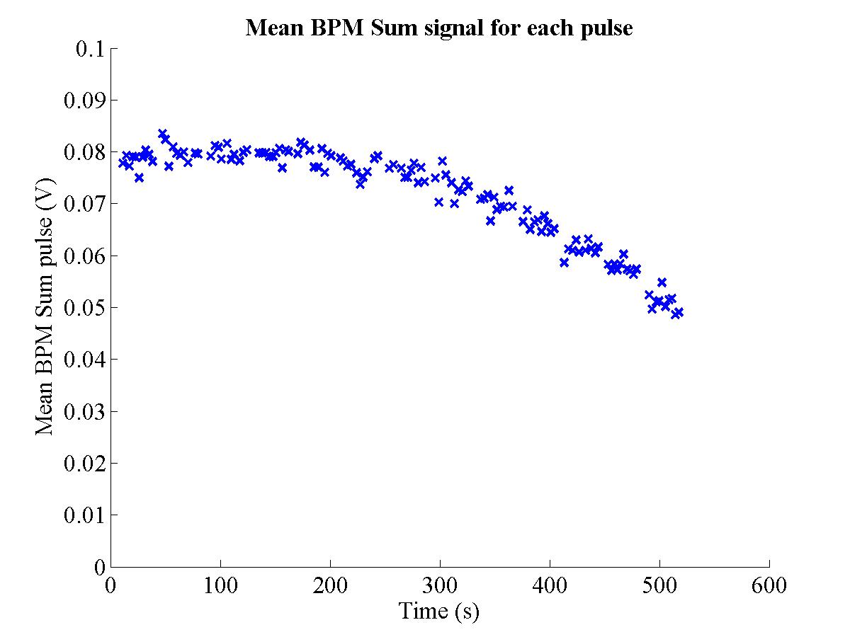
|
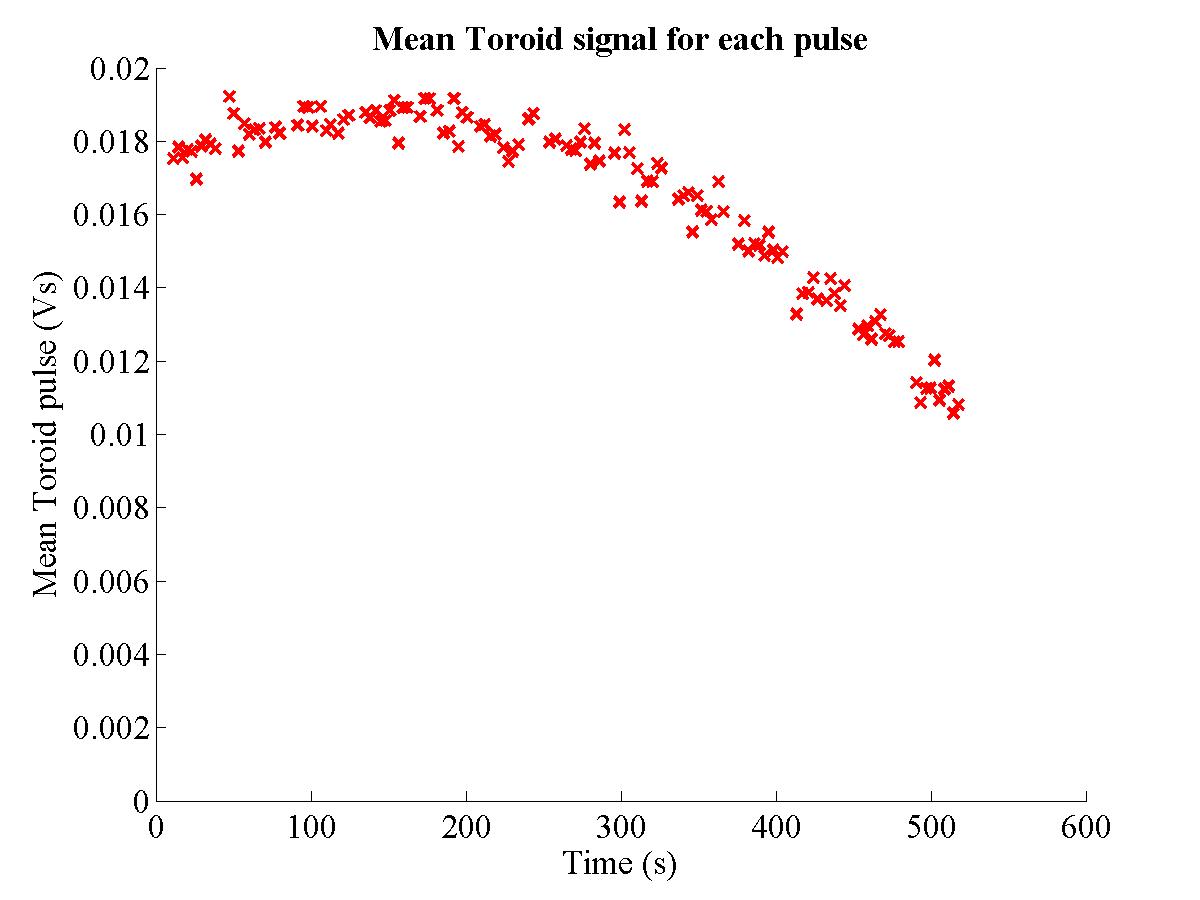
|
||||
| (a) Mean sum signal | (b) Mean toroid output | ||||
| |||||
In an attempt to measure the quality of the position measurement of the FONT BPM for the long pulse, the SCP was set up to steer the beam with dipole YCOR 1650 (see Fig. 4.32). 10 beam pulses were recorded for 13 field settings of YCOR 1650, with a variation between settings of 0.5 G-m. Both the integrated dipole field and the position measurement of stripline BPM 1761 were recorded. The resulting normalised beam positions are shown in Fig. 4.55. It is obvious at first glance that the pulse shape is repeatable from pulse to pulse: it also provides more evidence that the performance of the BPM processor is sound49. In order to correlate the normalised beam position with the dipole field, the mean of each pulse was taken between 320 ns and 440 ns: this is the region in which the pulse was considered to be stable and repeatable. A plot of the mean normalised position vs. the integrated field of YCOR 1650 for each pulse can be seen in Fig. 4.56. The position response shown in this figure is clearly an improvement over the short pulse position response (Fig. 4.37).
| Figure 4.58: The normalised BPM output for the long pulse beam as a function of the integrated field of YCOR 1650, using the first 8 dipole settings shown in Fig. 4.56. The red line is a line of best fit produced through a χ2 minimisation. |
It would appear from this plot that the normalised FONT BPM output has a nonlinear response to beam position, since it deviates above the line of best fit in the centre and falls below it towards either end. However, the larger integrated field of the dipole, and the associated normalised position measurement, correspond to a rapid fall off of the beam charge, as can be seen in Fig. 4.57. This figure shows the variation of the beam charge as a function of the time at which the measurement was made: note that there is a rapid deterioration in the beam charge after 300 s. This deterioration could be a result of the beam scraping on the aperture of the FONT BPM, the slope of the curve corresponding to the size of the aperture50. It could also be a result of the general deterioration in the quality of the beam. When the length of the long pulse beam was extended beyond ~150 ns, it was repeatedly observed to remain stable only for about 3 minutes before starting to deteriorate. If Fig. 4.56 is re-plotted with just the earlier data (corresponding to the first 8 dipole settings), a much better fit is obtained: this is shown in Fig. 4.58. The fit is clearly better than that shown in Fig. 4.56 as a result of using the high beam charge data. From this figure, a variation in normalised FONT BPM position of 0.323 normalised units (BPM units) per Gauss-metre of YCOR 1650 integrated dipole current is obtained.
| Figure 4.59: The normalised BPM output for the long pulse beam vs. the position measured by stripline BPM 1761. 13 beam positions were recorded, with 10 beam pulses at each position. The red line is a line of best fit produced through a χ2 minimisation. |
| Figure 4.60: The beam position measured by NLCTA stripline BPM 1761 as a function of the integrated field of dipole YCOR 1650. 13 beam positions were recorded, with 10 beam pulses at each position. The red line is a line of best fit produced through a χ2 minimisation. |
The final stage in measuring the position response of the FONT BPM to the long pulse beam is to compare the position as measured by stripline BPM 1761 to the normalised FONT BPM position. The beam position measured by BPM 1761 is shown plotted against the normalised FONT BPM position in Fig. 4.59. As one would expect, given the response shown in Fig. 4.58, the correlation between the two is again linear, to a good approximation. Again some nonlinear behaviour is evident further away from the centre of the beampipe. However, by comparing this plot to Fig. 4.60, which shows the response of BPM 1761 as a function of the integrated field of YCOR 1650, it is likely that the main source of this nonlinearity is the stripline BPM response. The data in Fig. 4.60 shows the same ‘S-bend’ shape as that in Fig. 4.59: since this is not present in Fig. 4.58, it is probable that this is a result of the stripline BPM response and not the X-band BPM. It is therefore likely that the X-band BPM has a long pulse position response that is very close to linear, for a beam that is close to its electrical centre.
By examining the data in Fig. 4.59, it is possible to relate the normalised position variation of the FONT BPM to the actual position variation as measured by stripline BPM 1761: a normalised position of 0.299 ± 0.012 BPM units = 1 mm for the fit to the data in Fig. 4.6051. It is also possible to put an upper limit on the precision of the normalised position measurement from the r.m.s. spread on each position. Since this position spread is likely to be dominated by beam jitter, rather than the precision of either BPM, the lowest r.m.s. position variation for each dipole setting is used. The minimum r.m.s. jitter on the stripline position is 22 microns (for the positions measured at~1 mm offset). The corresponding minimum jitter for the FONT BPM normalised position is 0.0069 BPM units which, using the previously measured scale for the normalised position variation corresponds to an r.m.s. jitter of 23 microns. Note that both these values are smaller than the previously measured beam jitter shown in Fig. 3.26. Given the sensitivity of the beam variation over a timescale of minutes, as noted above, it is likely that the beam jitter is closely related to the beam quality.
In Section 4.7.2, an explanation was given for the double peaked signal overshoot that appears on the difference signal for the short pulse beam. The implication is that such an effect should also be seen to some degree in the long pulse beam response. Although it is unclear from the data presented in Section 4.8.2, a clear example of this signal overshoot was observed on the difference signal for a number of sets of data. One example of such a signal is shown in Fig. 4.61, with the accompanying toroid signal in Fig. 4.62. Note that, at around 60 ns into the pulse the charge drops sharply on the toroid output. A corresponding drop is apparent on the X-band BPM difference signal, but instead of getting close to zero and then rising again, the BPM signal actually crosses over zero, becoming positive, before returning to its large negative value. A similar overshoot appears at the end of the pulse around 120 ns. The hypothesis was that the cause of the double peaks in the short pulse data was also the cause of the overshoots that one sees in the long pulse data i.e. that the incorrect cancellation occurring from the time difference in the signal paths causes the X-band BPM signal to overshoot.
| Figure 4.61: The BPM difference signal for a single pulse of the long pulse beam. Note the overshoot that appears at 60 ns and 120 ns as a result of the inexact signal cancellation. |
| Figure 4.62: The output of the toroid for the same pulse shown in Fig. 4.61. Note the location of the dips in the charge profile at 60 ns and 120 ns. |
| Figure 4.63: The simulated X-band BPM raw pickoff signals used to simulate the difference signal shown in Fig. 4.61. The blue trace represents the top pickoff signal and the red trace the bottom pickoff signal; relative time delay between signals is 0.5 ns. |
| Figure 4.64: The simulated X-band BPM difference signal using the two pulses shown in Fig. 4.63. Note the similarity to the actual difference signal shown in Fig. 4.61. |
To produce a facsimile of the actual pulse that arrives at the X-band BPM electronics, one of the recorded toroid signals was used to replicate the pickoff signals. Due to the relatively coarse granularity of the pulse as a result of the finite sampling rate of the scope, the bottom pulse was delayed in relation to the top pulse by some 0.5 ns; as before, the magnitude of the bottom signal was increased by 10% to simulate a beam off-centre (for comparison with the data). Again, these figures probably reflect some modicum of realism: although 0.5 ns is ten times longer a delay than one sees with a single half cycle delay at X-band (the actual figure is probably, given the relative signal path lengths of the processor used at the time, in the region of two and a half cycles, or 220 ps) the general effect of introducing a delay should still stand. As before, the signals were multiplied with an 11.424 GHz signal, subtracted and downmixed to DC with another 11.424 GHz signal; the raw signals can be seen in Fig. 4.63. The resulting signal is shown in Fig. 4.64: this shows the simulated position signal produced using the aforementioned cancellation method. There is a clear similarity between this pulse shape and the true X-band BPM difference signal shown in Fig. 4.63: instead of dropping towards zero without overshooting, which is the case for the charge signals used as the signal source for this output, the simulated signal overshoots past zero at similar points to that seen in the real data. It is also interesting that overshoots occur only in response to the falling edge of the charge signal, as mentioned above.
The likely conclusion is therefore that the cause of these overshoots is the signal path difference used for the signal cancellation, necessary to provide the difference signal used for the position measurement. Since these overshoots appear when the charge distribution of the beam drops rapidly, it is important that the beam have as flat a charge profile as possible. There is always a suspicion that, where a rapid change in normalised beam position is also accompanied by a rapid change in the beam charge, that this is a result of the same overshoot effect rather than a true change in beam position. Close inspection of Fig. 4.53 reveals that the first 70 ns of the sum signal shows a trough in the charge distribution. As expected, there is a corresponding trough in the difference signal: however, the trough in the difference signal is more pronounced than that of the sum signal, leading to a replication of this shape on the normalised signal (Fig. 4.54). The same is true for each sharp feature that appears on the sum signal: it is replicated on the difference signal, but appears sharper, and therefore reappears on the normalised signal. The likely explanation for this behaviour is the 44 ps signal path difference, as explained above. As a result, it was necessary to tune the beam very carefully for the FONT beam tests (Chapter 5) in order that the charge profile was as flat as possible. This was made all the more difficult by the rapid deterioration of the quality of the beam. For future iterations of the BPM processing electronics it is recommended that an alternative processing scheme is employed in order to eradicate this overshoot phenomenon.
30 For example, in the SLC, the BPM processors used for the stripline BPM's, with ~10 cm strips (giving Fc ≈ 714 MHz), filter the signal at 30 MHz. This is significantly cheaper than filtering at 714 MHz, and given the large number of BPM's involved is the most cost-effective solution [83].
31 Kimball Physics part no. for spherical cube: MCF133-SC6-A.
32 BPM assembly and pickoff tuning procedure carried out by Gavin Nesom, Oxford University.
33 0 dBm = 1 mW. The relation between dBm and mW is: mW = 10(dBm/10) or 10log10(mW) = dBm.
34 Although the Gunn diode is not a diode in the strict sense, since the I-V behaviour is the same for both positive and negative applied voltage, it is this nonlinear behaviour, between Vpeak and Vvalley, that gives it its name.
35 Strictly speaking power can pass in both directions through an isolator, but the attenuation in the backwards direction is some four orders of magnitude higher than the forward direction: the measured attenuation for the isolators used was 1.3 dB for the forward direction and 41 dB for the backward. This enormous difference in signal attenuation gives the isolator its directional behaviour.
36 Power reduction factor = 10dB/10; voltage reduction is the square root of this value since P ∝ V2.
37 The definition of σ for the two pulse types is different: the Gaussian pulse uses the usual definition, with ~63% of the particles in the bunch contained within ±1σ; for the square pulse, σ is half the pulse width.
38 The 15 dB attenuator was used as the original 10 dB attenuator could not be located at the time the measurement was made. It is possible that the S11 loss for the 10 dB attenuator is smaller than that measured for the 15 dB attenuator, giving a value for the total attenuation closer to the measured reflection.
39 The 2-way Splitter/Combiners used were Pulsar Microwave 2-way stripline power dividers, part no.: PS2-16-450/8S [101].
40 The mixer output becomes nonlinear with an RF input greater than +5 dBm, as can be seen in Fig. 4.23.
41 All the phase shifters used were MCE/Weinschel coaxial phase shifters; model no.: 980-4 [102].
42 The isolators used were Nova Microwave connectorized SMA isolators, model no.: 1070IES [103].
43 The 4-way Splitter/Combiner used was a Pulsar Microwave 4-way stripline power divider, part no.: PS4-12-452/7S [105].
44 One of this pair of phase shifters is essentially redundant, since only one is required to adjust the relative phase between the two signal paths. However, since both the phase and signal attenuation of both paths had to be exactly matched, it is much simpler to achieve this with a pair of identical phase shifters.
45 Due to the multiplication process of the mixer, two completely in phase signals of identical frequency produce a maximally positive output; for a 180° phase difference the output is maximally negative. A phase difference of ±90° between the two signals produces no output.
46 The signal was made maximally negative, rather than positive, since the BPM was required to produce a negative output if the beam was low of centre, and a positive output if the beam was high of centre.
47 It is possible that the stripline BPM response may become nonlinear for a beam that is a significant fraction of the beampipe diameter away from the centre [30,61]. A dipole magnet, however, should show no such nonlinearity, so the fact that such a clear linear response is evident in Fig. 4.38 is an excellent indication that the position as measured by the BPM is correct.
48 Roughly speaking, a 10% signal difference of this nature corresponds to a 10% larger signal pickup on one pickoff with respect to the other i.e. the beam is closer to one pickoff by 10% of the pickoff spacing. For a cavity size of 35 mm, this corresponds to a beam off-centre by 1.67 mm, not an unreasonable figure given the range shown in Fig. 4.38.
49 At least, if there are problems with the BPM processor that are causing the appearance of these artefacts in the normalised position measurement, they are certainly repeatable.
50 A number of attempts were made to produce a complete 2-D profile scan of the aperture of the beampipe of the FONT BPM using the integrated charge measured by the toroid and the BPM sum signal. However, due to the rapid deterioration of the beam, even over the course of a couple of minutes, coupled with the length of time required to record the position measurements and change the magnet currents, it proved impossible to do so.
51 The error is calculated from the mean r.m.s. spread of the position measurements shown in Fig. 4.59.
© Simon Jolly 2003