The approach used is to perform a ![]() fit between the SDM elements
measured in the data with the predictions made using fully simulated Monte
Carlo with different TGC values.
fit between the SDM elements
measured in the data with the predictions made using fully simulated Monte
Carlo with different TGC values.
The simple form of a ![]() [99] is given by:
[99] is given by:
Here ![]() is the measured value of an observable corresponding to a precise
value of
is the measured value of an observable corresponding to a precise
value of ![]() ,
,
![]() is the error on that value and
is the error on that value and
![]() is
the theoretical value corresponding to a precise value of
is
the theoretical value corresponding to a precise value of
![]() and is a function of the parameter that is being measured,
and is a function of the parameter that is being measured,
![]() . The
. The ![]() is formed by the sum over all the measured values,
is formed by the sum over all the measured values, ![]() , of
the observables.
, of
the observables.
In this context
![]() is the measured value of the SDM element in bin
is the measured value of the SDM element in bin ![]() of
of
![]() . The
theoretical value of the SDM element in bin
. The
theoretical value of the SDM element in bin ![]() , corresponding to
, corresponding to
![]() ,
is a function of the TGC parameter being measured.
The error,
,
is a function of the TGC parameter being measured.
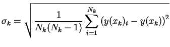
The error,
![]() , is the standard deviation on the mean of the measured
SDM element in bin
, is the standard deviation on the mean of the measured
SDM element in bin ![]() . The standard deviation on the mean is given by equation 6.2
. The standard deviation on the mean is given by equation 6.2
Where
![]() is the measured value from event
is the measured value from event ![]() and
and ![]() is
the mean
value of all events. In effect, the projection operator
is
the mean
value of all events. In effect, the projection operator
![]() applied to a single event gives the single measurement
applied to a single event gives the single measurement
![]() .
The form of equation 6.2
to calculate the statistical error on each SDM element for each bin
of
.
The form of equation 6.2
to calculate the statistical error on each SDM element for each bin
of
![]() is therefore given by equation 6.3.
is therefore given by equation 6.3.
![]() (i.e.
(i.e.
![]() )
represents the projection operators given in equation 4.1 and
)
represents the projection operators given in equation 4.1 and
![]() (i.e.
(i.e. ![]() ) is the calculated SDM
element.
The
) is the calculated SDM
element.
The ![]() given in
equation 6.1 is formed by the sum over all observables. Each SDM
element is separated into N bins of
given in
equation 6.1 is formed by the sum over all observables. Each SDM
element is separated into N bins of
![]() , so effectively
represents N observables. As there are nine SDM, it would also seem sensible
to sum over all these, so the
, so effectively
represents N observables. As there are nine SDM, it would also seem sensible
to sum over all these, so the ![]() would have the form shown in equation 6.4.
would have the form shown in equation 6.4.
Due to the hermitian nature of the spin density matrix,
![]() ,
not all the elements of the matrix are independent observables.
In fact, only the diagonal elements (
,
not all the elements of the matrix are independent observables.
In fact, only the diagonal elements (![]() ,
, ![]() and
and ![]() ) and three of the
off-diagonal elements,
) and three of the
off-diagonal elements, ![]() (=
(=
![]() ),
), ![]() (=
(=
![]() ) and
) and ![]() (=
(=
![]() ) need
be included in the
) need
be included in the ![]() fit.
fit.
The diagonal matrix elements are purely real and so represent three
observables.
However, as seen earlier, ![]() ,
, ![]() and
and ![]() are complex, so have both real
and imaginary
parts. Each of these then effectively represents 2 observables, the coefficient
of
the real part and that of the imaginary. This then totals nine observables to
which the
are complex, so have both real
and imaginary
parts. Each of these then effectively represents 2 observables, the coefficient
of
the real part and that of the imaginary. This then totals nine observables to
which the ![]() fit can be performed:
fit can be performed:
The imaginary SDM observables are completely insensitive to the CP-conserving couplings and are therefore not used when fitting these couplings. When fitting the CP-violating couplings all nine observables are used.
The ![]() given in equation 6.4 is a naive
simplification that assumes each measured SDM element is completely
uncorrelated from all the other SDM elements. All SDM elements in a
given in equation 6.4 is a naive
simplification that assumes each measured SDM element is completely
uncorrelated from all the other SDM elements. All SDM elements in a
![]() bin are derived from the same data subset and are therefore correlated.
The diagonal elements of the SDM are normalised to unity, so are
highly correlated. Correlations between different bins of
bin are derived from the same data subset and are therefore correlated.
The diagonal elements of the SDM are normalised to unity, so are
highly correlated. Correlations between different bins of
![]() may
be assumed to be negligible as they use different subsets of the data sample.
The correlation can be included in
equation 6.4 by introducing a covariance
matrix, as shown in equation 6.66.1.
may
be assumed to be negligible as they use different subsets of the data sample.
The correlation can be included in
equation 6.4 by introducing a covariance
matrix, as shown in equation 6.66.1.
In equation 6.6 the ![]() and
and ![]() represent the
nine SDM
observables indicated in equation 6.5. The covariance matrix,
represent the
nine SDM
observables indicated in equation 6.5. The covariance matrix,
![]() , is given by:
, is given by:
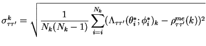
Where
![]() is the correlation between SDM observable
is the correlation between SDM observable ![]() and
and ![]() in bin
in bin ![]() of
of
![]() . A statistical analysis can be applied
to the data to directly calculate the covariance matrix:
. A statistical analysis can be applied
to the data to directly calculate the covariance matrix:
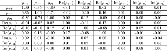
Table 6.1 shows the correlations between all
the SDM observables in one bin of
![]() , calculated from a SM sample of
EXCALIBUR Monte Carlo data. The SDM elements were divided into eight equal bins in
, calculated from a SM sample of
EXCALIBUR Monte Carlo data. The SDM elements were divided into eight equal bins in
![]() . The results shown are for the first bin. The correlations for the other
seven bins are of similar magnitude. It was found that the intra-bin
correlations were negligible.
. The results shown are for the first bin. The correlations for the other
seven bins are of similar magnitude. It was found that the intra-bin
correlations were negligible.
 |
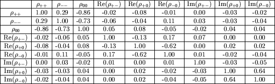
It was found that the correlations for non-Standard Model Monte Carlo were
similar to those in table 6.1, although not identical.
An example with Monte Carlo generated with an anomalous coupling of
![]() =
=![]() 2
is shown in table 6.2.
2
is shown in table 6.2.
 |
![$\displaystyle \chi^{2} = \sum^{N}_{k=1}\left[\frac{y(x_{k})-f(x_{k};a)}{\sigma_{k}}\right]^{2}$](img615.gif)
![$\displaystyle \chi^{2} = \sum^{N}_{k=1}\sum^{1}_{\tau=-1}\sum^{1}_{\tau^{\prime...
...)-\rho^{th}_{\tau\tau^{\prime}}(k;a)}{\sigma_{\tau\tau^{\prime}}(k)}\right]^{2}$](img627.gif)
![$\displaystyle \chi^{2} = \sum^{N}_{k=1}\sum^{9}_{i=1}\sum^{9}_{j=1} \left[ \lef...
...}_{ij}(k)\right) \left( \rho^{me}_{j}(k)-\rho^{th}_{j}(k;a) \right) \right]^{2}$](img638.gif)
![$\displaystyle V_{ij} = \frac{1}{N_{k}(N_{k}-1)} \left[ \sum_{\epsilon=1}^{N_{k}...
...heta^{*}_{\epsilon};\phi^{*}_{\epsilon})_{k} - \rho^{me}_{j}(k) \right) \right]$](img645.gif)