

High Speed TCP
Review and Implementation - September 9th 2002
Goal
To understand, implement and test the High Speed TCP protocol and suggest improvements.
Background
The main hstcp website can be found here.
Tom Duningan has implemented it with web100 here.
Excel spreadsheet with graphs and equations of HSTCP stuff here.
The Sally Floyd HSTCP modifications are based on the Response function of TCP:

Where T is the number of packets and s is the packet size.
From: Padhye et al. Modelling TCP Throughput - A Simple Model and its Empirical Validation 1998
By factoring out the second part of the denominator, we get,
- T = s/RTT*sqrt(2p/3) (1)
Where 2/3 is derived from the AIMD(0.5,1) a and b parameters of normal TCP.
(1) is the same as
- B = sqrt(3/2)/sqrt(p) (2)
packets per round trip time (ppr), where B is the actual throughput.
Using the bandwidth delay product,
- window = bandwidth * rtt / packet_size (3)
And factorising for bits instead of bytes
- window = bandwidth x rtt / (8 * packet size)
Assuming that the window size is directly proportional to the bandwidth, we can use (2) to get:
- window = sqrt(3/2)/sqrt(p) (4)
- window^2 = (3/2)/p
Which means that the loss rate, p is;
- p=(3/2)/window^2 (5)
The number of packets between losses is just the inverse of the loss rate, ie
- #pkts_between_losses = 1/p
- #pkts_between_losses = window^2/(3/2) (6)
The actual time between losses is then a matter of dividing (6) by the congestion window after multiplying it by the rtt
- time between losses = ( rtt * #pkts between losses) / window ???
these ultimately lead to the fact that hte throughput is limited by two factors: the loss of packets and the window size.
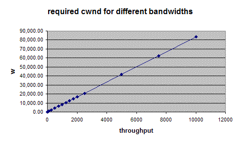 |
This graph shows the relationship between the congestion window and the throughput achieveable given a constant rtt and packet size |
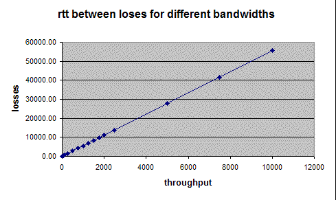 |
This graph shows the number of packet per rtt that we need between losses in order to achieve the throughput indicated. |
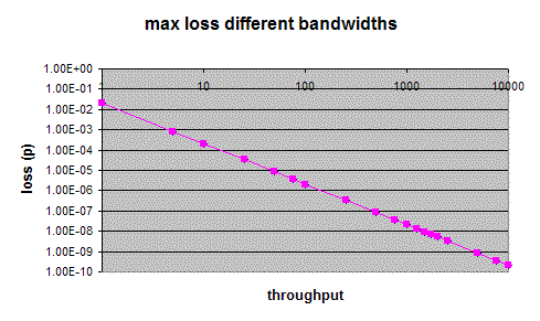 |
This grpah shows the loss rate that we need in order to achieve the indicated throughput. |
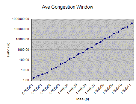
The HSTCP model makes assumptions on the achieveable loss rates on a system. Therefore, we must understand the relationship between the loss rate and the window size of a tcp system.
Given (4), ie
- window = sqrt(3/2)/sqrt(p)
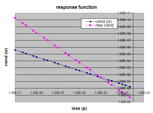
we can plot the following:
From this relation we can go about formulating a new response function for HSTCP. We need to consider 4 variables:
| Low_Window | The size of the congestion window whereby we switch regimes from the Standard TCP to the HSTCP implementation |
| High_Window | The size of the congestion window for the relevant bandwidth required for optimal performance at high throughputs |
| Low_P | Defines the Lowest loss rate expected for HSTCP - ie the relevent loss rate for the Low_Window |
| High_P | The corresponding loss rate for High_Window |
With this, we ca define the new response function as:
- w' = (p/Low_P)^S Low_Window (7)
where
- S = (LOG(High_Window)-LOG(Low_Window))/(LOG(High_P)-LOG(Low_P))
if we specify the following parameters:
| Low_Window | 38 | |
| High_Window | 833333.3333 | |
| Low_P | 1.00E-03 | |
| High_P | 0.0000001 |
We get the following response function:
Mapping to values of a and b
| Thu, 7 August, 2003 3:24 |
Room D14, High Energy Particle Physics, Dept. of Physics & Astronomy, UCL, Gower St, London, WC1E 6BT